Automated Reports with Parameters
Geological Automated web base reports
By Alonso Otiniano in Geoscience Water Resource R
December 26, 2021
¿What is an automated report with parameters?
Well, in simple terms an automated report is a document in any format (.docx, .ppt, .pdf, .html and so on) that can be update in a specific time window iteratively while is required, in the case refer to parameters, there are some variables that can be change, for example, basin, sub-basin, department, province, geological horizont, lake, etc. (espacial) and hourly, daily, monthly , etc. (time) or another kind of variable that can be update following the particular requirements of the data analysis in geology.
Advantages of Automated Report with parameters
-
Reduce the time and men-hours in analysis an processing, that helps to carry fast response in order to be more productive for reducing risk, vulnerability or similar activities.
-
Improve la quality of communication between scientist and applied engineering in order to make decision to achieve common goals in a project.
Disadvantages
- Preparation and high-level programming skills combined with the expertise in this case of the geological kwondledge.
Method (¿How it works?)
The example that I am going to show you is base on Hydrological data, so the parameters are related to variables in a dataset (parameters to uso for modeling), but some variables are not use like a parameters to change the final output process of the automated mapping and analysis report.
The method consist in create two structural blocks, that blocks work sincronicaly to make the automated report (in this case semi-automated), that contain the following to parts:
Inner Redactor
This the code made in R and Javascript to keep the system of libriries, the yaml, and many inner parts that works to create the setting procedure, I will show the basic part of the code (I do not want to scared you :D, is really simple):
title: "Modulo Peligros Geológicos - Aspectos Generales "
author: "A.Otiniano"
date: "03 March, 2023"
output:
  prettydoc::html_pretty:
params:
  distrito: NA
  provincia: NA
  region: NA
  sector: NA
  peligro: NA
  zona: NA
  ubicacion: NA
  difae:
    label: "Factor Comparacion"
    value: mayor
    input: select
    choices: ["mayor","menor","igual"]
  long: -77.01
  lat: -9.30
  date01: as.Date(x = "2021-12-01", format = "yy/mm/dd")
  date02: as.Date(x = "2021-12-04", format = "yy/mm/dd")
The package to developed are:
library(tidyverse); library(readr); library(lubridate); library(leaflet.extras)
library(plotly); library(nasapower); library(leaflet); library(leafem)
library(htmltools); library(mapview)
The code developed using R and Javascript is too long, so I do not included the whole script here, but if you want to know the hole code, only contact me and I will very pleased to share with you :D.
The second part is the Frontend for the user, let´s see:
Frontend User
The enviroment for the final user, in this case, the research geology interact with the report to generate. This enviroment is created by a side bar like panel, where join up the variables inputs of the model. To the right side, is found the central panel, where was generated the map to be able to located the select dot, moreover the integration of inner functions of geospatial objects. A fragment of the code is showing below:
### Panel and Buttons

ui <- bootstrapPage(
    sidebarLayout(
      sidebarPanel(
        id = "inputs",
    textInput("distrito", h4("distrito"), value = "Entrar distrito ..."),
    textInput("provincia", h4("provincia"), value = "Entrar provincia ..."),
    textInput("region", h4("region"), value = "Entrar region ..."),
    textInput("sector", h4("sector"), value = "Entrar sector ..."),
    textInput("peligro", h4("peligro"), value = "Entrar peligro ..."),
    textInput("zona", h4("zona"), value = "Entrar zona ..."),
    textInput("ubicacion", h4("ubicacion"), value = "Entrar ubicación ..."),
    checkboxGroupInput("difae", "difae", c("mayor"="mayor","menor"="menor",
    "igual"="igual")),
    numericInput("long","longitud", value = -77.01),
    numericInput("lat","longitud", value = -9.30),
    numericInput("graticula", "graticula", value = 5),
    dateInput("date01", "Inicio:", value = "2021-12-01", format = "yy/mm/dd"),
    dateInput("date02", "Fin:", value = "2021-12-04", format = "yy/mm/dd"),
    downloadButton("report", "Generate report"), width = 2
  ),
  mainPanel(selectInput("selector", "Que capturo?",
                                c("Entire page" = "body", "map" = "#map",
                                "Inputs" = "#inputs")),
                    textInput("filename", "File name", "screenshot"),
    actionButton("action", "Toma Captura", icon("camera"), class = "btn-success"),
              leafletOutput("map", height="750"),  #height="100vh"
              downloadButton(outputId = "dl"), width = 10)))
The code for the map with the saving systems is large, in the next script I will show yoy the most important parts:
### Map

output$map <- renderLeaflet({
    input$goButton
    leaflet() %>%
      addTiles(group = "Street View") %>%
      addProviderTiles("OpenStreetMap",group = "OpenStreetMap") %>%
      addProviderTiles("Stamen.Toner",group = "Stamen.Toner") %>%
      addProviderTiles("Stamen.Terrain",group = "Stamen.Terrain") %>%
      addProviderTiles("Esri.WorldStreetMap",group = "Esri.WorldStreetMap") %>%
      addProviderTiles("Wikimedia",group = "Wikimedia") %>%
      addProviderTiles("CartoDB.Positron",group = "CartoDB.Positron") %>%
      addProviderTiles("Esri.WorldImagery",group = "Esri.WorldImagery") %>%
      addGraticule(group = "Graticule", interval = input$graticula) %>%

      addMarkers(lng = input$long, lat = input$lat, icon = greenLeafIcon) %>%
      addMeasure(
        position = "bottomleft",
        primaryLengthUnit = "meters",
        primaryAreaUnit = "sqmeters",
        activeColor = "#0bd3d3",
        completedColor = "#f890e7"
      ) ... continua

### Screen Photo

  code <- reactive({
    if (input$selector == "body") {
      selector <- ""
    } else {
      selector <- paste0('  selector = "', input$selector, '",\n')
    }
    paste0(
      'screenshot(\n',
      selector,
      '  scale = ', input$scale, ',\n',
      '  filename = "', input$filename, '"\n',
      ')'
    )
  })

  observeEvent(input$action, {
    eval(parse(text = code()))
  })
You can see in the next to pictures a photo of the app running:
knitr::include_graphics(path = "Inputs.png")
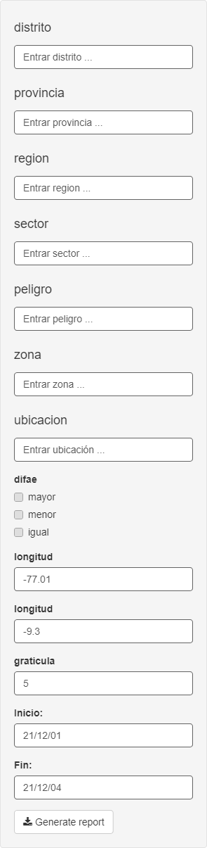
Figure 1: Inputs
knitr::include_graphics(path = "Mapa.PNG")
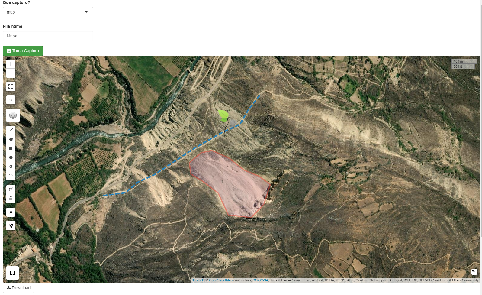
Figure 2: Central Map
At last but not least important is the communication between the inner redactor and the frontend, so let´s see it:
Inner Redactor and Frontend
The basic code is showing below:
### Conecction

    output$report <- downloadHandler(

      filename = "report.html",
      content = function(file) {

        tempReport <- file.path(tempdir(), "report.Rmd")   # tempdir() tenia esta direccion ahora cambiare.
        file.copy("report.Rmd", tempReport, overwrite = TRUE)

       params <- list(long = input$long, difae = input$difae, ubicacion = input$ubicacion,
                       lat = input$lat, date01 = input$date01, date02 = input$date02,
                       distrito = input$distrito, provincia = input$provincia,
                       region = input$region, sector = input$sector, peligro = input$peligro,
                       zona = input$zona)

        rmarkdown::render(tempReport, output_file = file,
                          params = params,
                          envir = new.env(parent = globalenv())
        )
      }
    )
This code allow connect the two parts and works in an efficient way in the application created.
Well that is all, not to complicate, no?
I am going to show you some photos of the application working, soon I hosted in an developed enviromment to all of you can see it.
knitr::include_graphics(path = "inputs_elegidos.png")
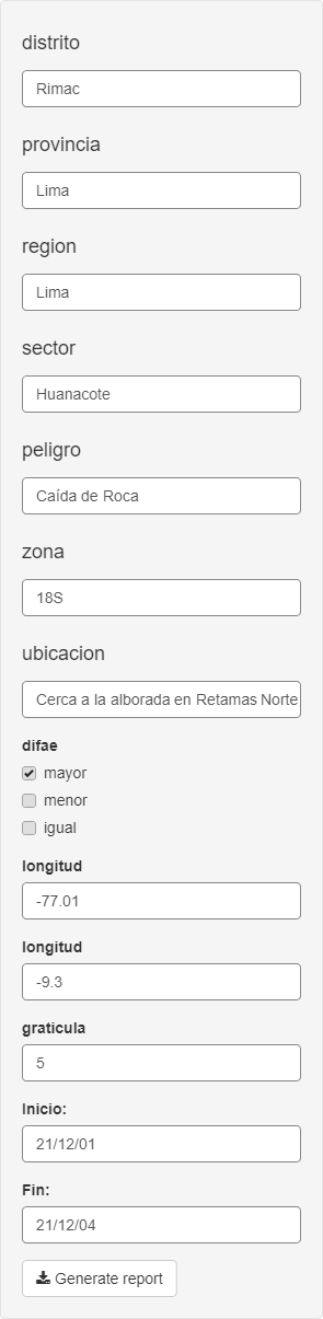
Figure 3: Testing Inputs
We give click in generate report, and wait almost 30s to 1 minut, The report is obtained and we have the file (in this case .html) to use and enjoy it.
knitr::include_graphics(path = "Generar_report.png")
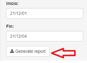
Figure 4: Document Generarted
knitr::include_graphics(path = "Repo01.PNG")
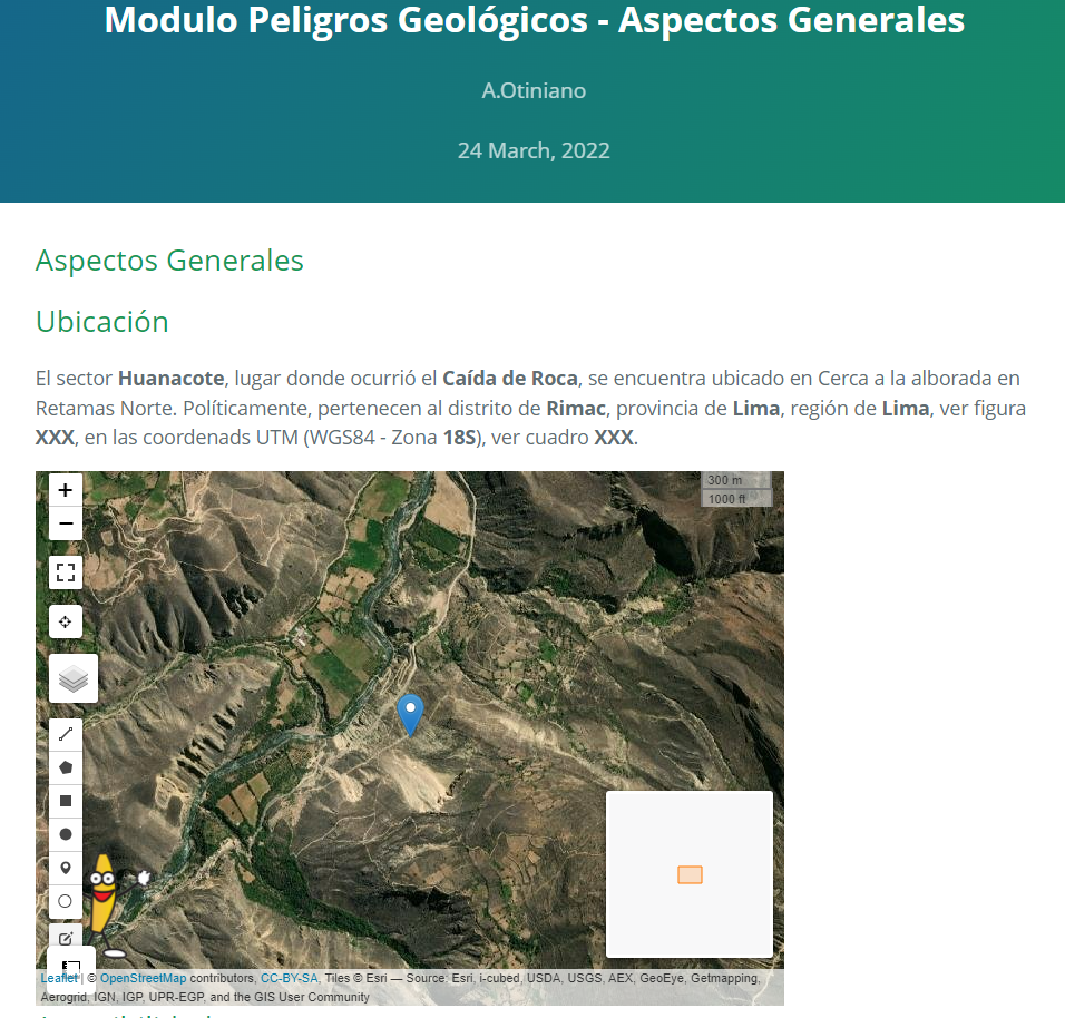
Figure 5: Location Map
knitr::include_graphics(path = "Repo02.PNG")
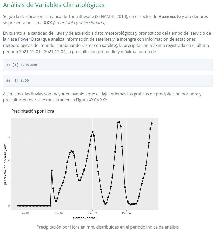
Figure 6: Climatological Variables Analysis 01
knitr::include_graphics(path = "Repo03.PNG")
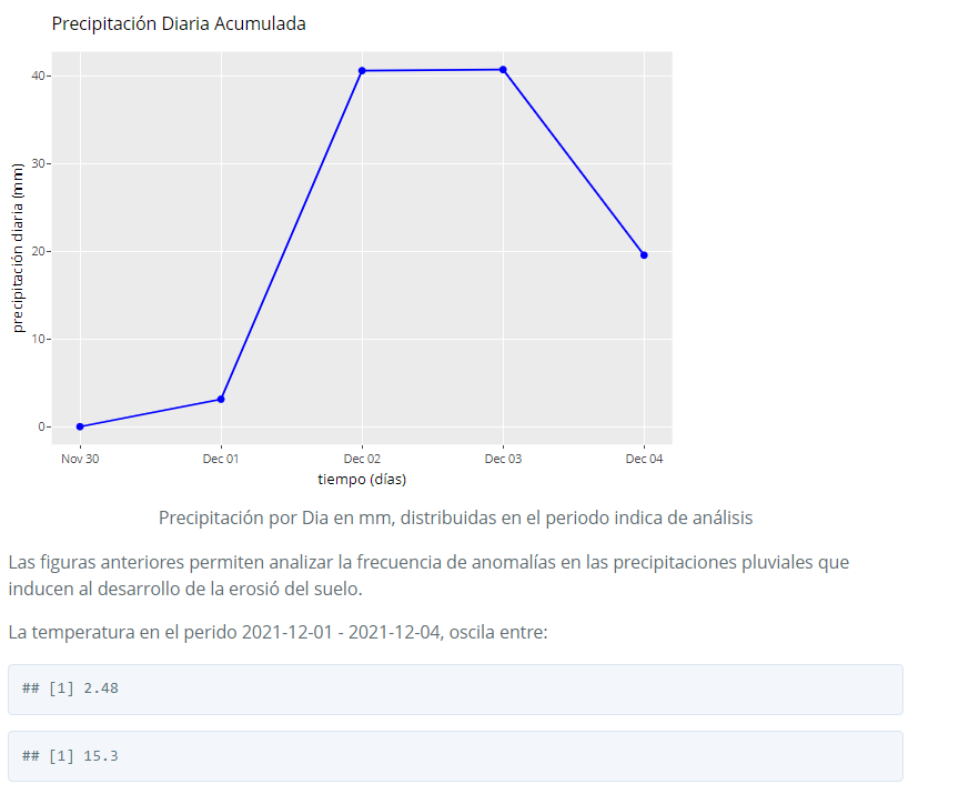
Figure 7: Climatological Variables Analysis 02
knitr::include_graphics(path = "Repo04.PNG")

Figure 8: Climatological Variables Analysis 03
Final Comments
- Zum Schluss (like you said “to finish” in German), the creating required some basics steps to works, the developed of a simple application can take few days or hours all depende of the database size and structure, so let´s try to do it, and if you can not, I will help you
!Geological Science for all!
Bibliography
Referencias Bibliográficas
https://bookdown.org/yihui/rmarkdown-cookbook/
https://www.oracle.com/technetwork/java/jvmls2013vitek-2013524.pdf