Surface Water Analysis - Non Spatial I
Subbasin Alto Camaná - Arequipa
By Alonso Otiniano in Water
December 27, 2021
- Data Base (Structure and General Review).
- Below Detection Limit Values (<L.D.).
- Exploratory Data Analysis usign statistics
- Conclusions:
- Recommendations:
- Bibliography:
Data Base (Structure and General Review).
It is recommendable to look up Cheetsheet Rstudio that contain many of the functions that we are going to use for the analysis. We are going to start loading the principal libraries (before you have to install the libraries).
knitr::opts_chunk$set(echo = TRUE, warning = FALSE, message=FALSE, fig.align = 'center')
#### Loading L ####
library(MASS)
library(NADA)
library(ggmap)
library(nortest)
library(psych)
library(chron)
library(readxl)
library(tidyverse)
library(knitr)
library(xaringan)
library(xaringanExtra)
xaringanExtra::use_panelset()dir() #verify directory## [1] "BD_AC.xlsx" "BD_AC_final.csv" "featured.jpg"
## [4] "index.html" "index.Rmd" "index.Rmd.lock~"
## [7] "index_files" "Sumario_Estiaje.csv"Loading Data:
To loading the data we have to use the function read_xlsx():
AC <- read_xlsx("BD_AC.xlsx", col_names = TRUE)
#View(AC)   Allow visualize data
dim(AC)  # dimensions of data frame
## [1] 161 169colnames(AC) # name of all the columns## [1] "Proyecto" "Temporada" "Codigo"
## [4] "Codigo_Corto" "Nombre" "Nombre_Completo"
## [7] "Fecha" "Hora" "Norte"
## [10] "Este" "Cota" "Zona"
## [13] "Lugar" "Distrito" "Provincia"
## [16] "Vertiente" "Cuenca" "Subcuenca"
## [19] "Microcuenca" "Tipo_Fuente" "Clase_Fuente"
## [22] "Uso" "PFQ" "T.Analisis"
## [25] "Muestreo" "Monitoreo" "Blanco"
## [28] "Estandar" "Duplicado" "Asp_Geologico"
## [31] "Desc_Litologica" "Morfologia" "Pendiente"
## [34] "Caudal" "Color" "Olor"
## [37] "T_Fuente" "T_Ambiente" "pH"
## [40] "pH_mV" "Eh" "ORP_mv"
## [43] "CE_uS_cm" "TDS_mg_L" "TDS_ppt"
## [46] "Salinidad_PSU" "Resistividad_Kohm-cm" "OD_mgL"
## [49] "OD_Sat." "Precipitados" "Algas_plantas"
## [52] "Basurales" "Animales" "Letrinas_Sítios"
## [55] "Poblacion" "Pasivos_Ambientales" "Act_Antropica"
## [58] "Alt.Geo.Nat" "Ev.Meteo" "Viento"
## [61] "Foto" "Observaciones" "Realizado_por"
## [64] "Alcalinidad_mgCaCO3_L" "CO3_menos_2_mg_L" "HCO3_menos"
## [67] "F" "Cl" "NO3_menos_1"
## [70] "NO3_menos_1_como_N" "SO4_menos_2" "NO2_menos_1"
## [73] "NO2_menos_1_como_N" "Na_dis" "Mg_dis"
## [76] "K_dis" "Ca_dis" "Sr_dis"
## [79] "Li_dis" "Si_dis" "SiO2 _dis"
## [82] "Ag_dis" "Al_dis" "As_dis"
## [85] "B_dis" "Ba_dis" "Be_dis"
## [88] "Bi_dis" "Cd_dis" "Ce_dis"
## [91] "Co_dis" "Cr_dis" "Cu_dis"
## [94] "Fe_dis" "Hg_dis" "La_dis"
## [97] "Mn_dis" "Mo_dis" "Ni_dis"
## [100] "Pb_dis" "S_dis" "Sb_dis"
## [103] "Se_dis" "Sn_dis" "Th_dis"
## [106] "Ti_dis" "Tl_dis" "U_dis"
## [109] "V_dis" "W_dis" "Y_dis"
## [112] "Zn_dis" "Na_tot" "Mg_tot"
## [115] "K_tot" "Ca_tot" "Sr_tot"
## [118] "Li_tot" "Si_tot" "SiO2_tot"
## [121] "Ag_tot" "Al_tot" "As_tot"
## [124] "B_tot" "Ba_tot" "Be_tot"
## [127] "Bi_tot" "Cd_tot" "Ce_tot"
## [130] "Co_tot" "Cr_tot" "Cu_tot"
## [133] "Fe_tot" "Hg_tot" "La_tot"
## [136] "Mn_tot" "Mo_tot" "Ni_tot"
## [139] "Pb_tot" "S_tot" "Sb_tot"
## [142] "Se_tot" "Sn_tot" "Th_tot"
## [145] "Ti_tot" "Tl_tot" "U_tot"
## [148] "V_tot" "W_tot" "Y_tot"
## [151] "Zn_tot" "Ca_meq_l" "Mg_meq_l"
## [154] "Na_meq_l" "K_meq_l" "Total_meq_l.1"
## [157] "HCO3_meq_l" "CO3_meq_l" "SO4_meq_l"
## [160] "Cl_meq_l" "Total_meq_l.2" "BI_per"
## [163] "Ca_per" "Mg_per" "Na_plus_K_per"
## [166] "HCO3_plus_CO3_per" "SO4_per" "Cl_per"
## [169] "HIDROTIPO"With dim function we know that the data frame have 161 rows and 169 columns. Also the colnames function give us the name of all the columns variables.
str(AC[ ,-c(31,62)], list.len = ncol(AC[ ,-c(31,62)]), vec.len=4) #check all the structure of your data## tibble [161 x 167] (S3: tbl_df/tbl/data.frame)
## $ Proyecto : chr [1:161] "GA47C" "GA47C" "GA47C" "GA47C" ...
## $ Temporada : chr [1:161] "Avenida" "Avenida" "Avenida" "Avenida" ...
## $ Codigo : chr [1:161] "13491-19-GW-121" "13491-19-GW-134" "13491-19-GW-138" "13491-19-GW-141" ...
## $ Codigo_Corto : chr [1:161] "GW-121" "GW-134" "GW-138" "GW-141" ...
## $ Nombre : chr [1:161] "Ran Ran" "Belén" "Joyas" "Lari" ...
## $ Nombre_Completo : chr [1:161] "Manantial Ran Ran" "Geiser Belén" "Galería Filtrante Joyas" "Termal Lari" ...
## $ Fecha : POSIXct[1:161], format: "2019-04-25" "2019-04-27" ...
## $ Hora : POSIXct[1:161], format: "1899-12-31 12:14:00" "1899-12-31 09:42:00" ...
## $ Norte : num [1:161] 8289456 8273538 8269490 8269663 8269242 ...
## $ Este : num [1:161] 221441 178306 182249 203172 201755 ...
## $ Cota : num [1:161] 4463 2160 3408 3239 3284 ...
## $ Zona : chr [1:161] "19 S" "19 S" "19 S" "19 S" ...
## $ Lugar : chr [1:161] "Ran Ran" "Belén" "Joyas" "Lari" ...
## $ Distrito : chr [1:161] "Tuti" "Tapay" "Cabanaconde" "Lari" ...
## $ Provincia : chr [1:161] "Caylloma" "Caylloma" "Caylloma" "Caylloma" ...
## $ Vertiente : chr [1:161] "Pacífico" "Pacífico" "Pacífico" "Pacífico" ...
## $ Cuenca : chr [1:161] "Camaná" "Camaná" "Camaná" "Camaná" ...
## $ Subcuenca : chr [1:161] "Alto Camaná" "Alto Camaná" "Alto Camaná" "Alto Camaná" ...
## $ Microcuenca : chr [1:161] "Tuti" "Cabanaconde" "Cabanaconde" "Maca" ...
## $ Tipo_Fuente : chr [1:161] "Subterránea" "Subterránea" "Subterránea" "Subterránea" ...
## $ Clase_Fuente : chr [1:161] "Manantial" "Geiser" "Galería Filtrante" "Manantial" ...
## $ Uso : chr [1:161] "Ninguno" "Ninguno" "Consumo humano" "Ninguno" ...
## $ PFQ : chr [1:161] "Sí" "Sí" "Sí" "Sí" ...
## $ T.Analisis : chr [1:161] "Químico" "Químico" "Químico" "Químico" ...
## $ Muestreo : chr [1:161] "Original" "Original" "Original" "Original" ...
## $ Monitoreo : chr [1:161] NA NA NA NA ...
## $ Blanco : logi [1:161] NA NA NA NA NA NA ...
## $ Estandar : logi [1:161] NA NA NA NA NA NA ...
## $ Duplicado : chr [1:161] NA NA NA NA ...
## $ Asp_Geologico : chr [1:161] "Volcánico/Depósito superficial" "Volcánico/Depósito superficial" "Volcánico" "Volcánico/Depósito superficial" ...
## $ Morfologia : chr [1:161] "Planicie" "Valle encañonado" "Escarpa" "Valle Fluvial" ...
## $ Pendiente : chr [1:161] "Muy baja" "Baja" "Media" "Muy Baja" ...
## $ Caudal : num [1:161] NA 15 50 3 5 50 40 NA NA NA ...
## $ Color : chr [1:161] "Incoloro" "Incoloro" "Incoloro" "Incoloro" ...
## $ Olor : chr [1:161] "Inodoro" "Inodoro" "Inodoro" "Inodoro" ...
## $ T_Fuente : num [1:161] 18 85.5 19.3 32.1 19.4 16.7 15.7 37 74.8 42.9 ...
## $ T_Ambiente : logi [1:161] NA NA NA NA NA NA ...
## $ pH : num [1:161] 6.82 7.6 7.04 7.47 7.18 7.06 7.19 7 5.88 6.02 ...
## $ pH_mV : num [1:161] 7.4 44.3 5.2 3.9 13.3 19.4 13 10.1 60.9 39.9 ...
## $ Eh : logi [1:161] NA NA NA NA NA NA ...
## $ ORP_mv : num [1:161] 380 98.2 128.4 23.3 179.8 ...
## $ CE_uS_cm : num [1:161] 67.4 4111 336.7 823.4 210.2 ...
## $ TDS_mg_L : num [1:161] 33.7 2010 165.5 404 103.5 ...
## $ TDS_ppt : chr [1:161] NA NA NA NA ...
## $ Salinidad_PSU : num [1:161] 0.086 2.173 0.211 0.454 0.151 ...
## $ Resistividad_Kohm-cm : num [1:161] 14.67 0.244 2.97 1.214 4.758 ...
## $ OD_mgL : num [1:161] 7.84 NA 5.83 1.14 4 6.03 5.69 3.63 NA 1.91 ...
## $ OD_Sat. : num [1:161] 145.1 NA 101.8 23.5 65.1 ...
## $ Precipitados : chr [1:161] "No" "No" "No" "No" ...
## $ Algas_plantas : chr [1:161] "No" "No" "No" "No" ...
## $ Basurales : chr [1:161] "No" "No" "No" "Sí" ...
## $ Animales : chr [1:161] "No" "No" "Sí" "No" ...
## $ Letrinas_Sítios : chr [1:161] "No" "no" "No" "no" ...
## $ Poblacion : chr [1:161] "Rural" "Rural" "Rural" "Rural" ...
## $ Pasivos_Ambientales : chr [1:161] "No" "no" "no" "no" ...
## $ Act_Antropica : chr [1:161] "Ninguno" "Ninguno" "Ganadería" "Ninguno" ...
## $ Alt.Geo.Nat : chr [1:161] "No" "No" "No" "No" ...
## $ Ev.Meteo : chr [1:161] "Ninguno" "Ninguno" "Ninguno" "Ninguno" ...
## $ Viento : chr [1:161] "No" "No" "No" "No" ...
## $ Foto : chr [1:161] "524534" "611634" "646660" "669677" ...
## $ Realizado_por : chr [1:161] "I. Becerra y J. Ortiz" "I. Becerra y J. Ortiz" "I. Becerra y J. Ortiz" "I. Becerra y J. Ortiz" ...
## $ Alcalinidad_mgCaCO3_L: chr [1:161] "23" "54.5" "101.7" "166.8" ...
## $ CO3_menos_2_mg_L : chr [1:161] "<1" "1" "<1" "2" ...
## $ HCO3_menos : chr [1:161] "23" "53" "101" "165" ...
## $ F : chr [1:161] "<0.2" "5.2" "0.2" "0.5" ...
## $ Cl : chr [1:161] "0.3" "850.9" "1.4" "2.4" ...
## $ NO3_menos_1 : chr [1:161] NA NA NA NA ...
## $ NO3_menos_1_como_N : chr [1:161] NA NA NA NA ...
## $ SO4_menos_2 : num [1:161] 5.3 341.5 65.9 262.7 9.2 ...
## $ NO2_menos_1 : chr [1:161] NA NA NA NA ...
## $ NO2_menos_1_como_N : chr [1:161] NA NA NA NA ...
## $ Na_dis : num [1:161] 3.3 549.5 14.7 38.7 15.6 ...
## $ Mg_dis : num [1:161] 2.2 1.4 15.4 28.2 7.2 7.7 18.2 2.4 6.4 8.6 ...
## $ K_dis : num [1:161] 2 75.1 3.6 7.8 2.6 2 2.4 14.2 61.9 26.6 ...
## $ Ca_dis : num [1:161] 2.8 39.1 23.7 71.7 10.7 12.9 41.7 36.1 69.4 35.3 ...
## $ Sr_dis : num [1:161] 0.0293 1.0192 0.1783 0.7257 0.0889 ...
## $ Li_dis : chr [1:161] "6.9999999999999999E-4" "5.0960000000000001" "2.9700000000000001E-2" "2.1999999999999999E-2" ...
## $ Si_dis : num [1:161] 13.9 89.6 33.1 32.9 27 ...
## $ SiO2 _dis : num [1:161] 29.8 191.8 70.8 70.5 57.7 ...
## $ Ag_dis : chr [1:161] "<0.0003" "<0.0003" "<0.0003" "<0.0003" ...
## $ Al_dis : chr [1:161] "<0.005" "1.6E-2" "<0.005" "1.2E-2" ...
## $ As_dis : chr [1:161] "<0.001" "1.742" "7.0000000000000001E-3" "7.1999999999999995E-2" ...
## $ B_dis : chr [1:161] "<0.05" "16.12" "<0.05" "0.14000000000000001" ...
## $ Ba_dis : num [1:161] 0.0138 0.1355 0.0228 0.0341 0.0305 ...
## $ Be_dis : chr [1:161] "<0.0002" "<0.0002" "<0.0002" "<0.0002" ...
## $ Bi_dis : chr [1:161] "<0.0002" "<0.0002" "<0.0002" "<0.0002" ...
## $ Cd_dis : chr [1:161] "<0.0002" "<0.0002" "<0.0002" "6.4999999999999997E-3" ...
## $ Ce_dis : chr [1:161] "<0.0002" "<0.0002" "<0.0002" "<0.0002" ...
## $ Co_dis : chr [1:161] "<0.0002" "2.9999999999999997E-4" "<0.0002" "<0.0002" ...
## $ Cr_dis : chr [1:161] "<0.001" "<0.001" "<0.001" "1E-3" ...
## $ Cu_dis : chr [1:161] "<0.0005" "<0.0005" "5.9999999999999995E-4" "1.1999999999999999E-3" ...
## $ Fe_dis : chr [1:161] "0.01" "<0.01" "0.03" "0.19" ...
## $ Hg_dis : chr [1:161] "<0.020" "<0.020" "<0.020" "<0.020" ...
## $ La_dis : chr [1:161] "<0.0002" "<0.0002" "<0.0002" "<0.0002" ...
## $ Mn_dis : chr [1:161] "4.0000000000000002E-4" "8.9999999999999998E-4" "<0.0002" "0.27189999999999998" ...
## $ Mo_dis : chr [1:161] "4.0000000000000002E-4" "2.3E-3" "1.6999999999999999E-3" "1.2800000000000001E-2" ...
## $ Ni_dis : chr [1:161] "<0.0007" "<0.0007" "<0.0007" "<0.0007" ...
## $ Pb_dis : chr [1:161] "<0.0005" "<0.0005" "<0.0005" "5.9999999999999995E-4" ...
## $ S_dis : num [1:161] 1.8 115.1 22.1 88.2 3.2 ...
## $ Sb_dis : chr [1:161] "<0.0008" "9.01E-2" "<0.0008" "<0.0008" ...
## $ Se_dis : chr [1:161] "<0.002" "<0.002" "<0.002" "<0.002" ...
## $ Sn_dis : chr [1:161] "<0.0005" "<0.0005" "<0.0005" "<0.0005" ...
## $ Th_dis : chr [1:161] "<0.0002" "<0.0002" "<0.0002" "<0.0002" ...
## $ Ti_dis : chr [1:161] "1.2999999999999999E-3" "1.3599999999999999E-2" "2.8E-3" "<0.0006" ...
## $ Tl_dis : chr [1:161] "<0.0001" "6.1999999999999998E-3" "<0.0001" "<0.0001" ...
## $ U_dis : chr [1:161] "<0.0001" "<0.0001" "5.9999999999999995E-4" "<0.0001" ...
## $ V_dis : chr [1:161] "5.4999999999999997E-3" "6.7000000000000002E-3" "2.6100000000000002E-2" "<0.0005" ...
## $ W_dis : chr [1:161] "<0.0005" "7.9899999999999999E-2" "<0.0005" "<0.0005" ...
## $ Y_dis : chr [1:161] "<0.0005" "<0.0005" "<0.0005" "<0.0005" ...
## $ Zn_dis : chr [1:161] "6.0000000000000001E-3" "1.0999999999999999E-2" "7.0000000000000001E-3" "1.2999999999999999E-2" ...
## $ Na_tot : num [1:161] 3.4 614.9 16.7 44.3 17.6 ...
## $ Mg_tot : num [1:161] 2.5 1.8 17.9 34.8 8.6 9.3 21.4 2.8 7.7 10 ...
## $ K_tot : num [1:161] 2.1 80.5 4 8.5 3 2.2 2.6 15.7 71.7 30.5 ...
## $ Ca_tot : num [1:161] 3.1 41.7 26.9 86.1 12.6 15.4 48.2 37.8 77.4 38.5 ...
## $ Sr_tot : num [1:161] 0.0314 1.108 0.2023 0.733 0.0933 ...
## $ Li_tot : chr [1:161] "8.9999999999999998E-4" "5.7164000000000001" "3.04E-2" "2.2599999999999999E-2" ...
## $ Si_tot : num [1:161] 16.3 101.5 39.6 41.4 33.2 ...
## $ SiO2_tot : num [1:161] 34.9 217.3 84.7 88.5 71.1 ...
## $ Ag_tot : chr [1:161] "<0.0003" "<0.0003" "<0.0003" "<0.0003" ...
## $ Al_tot : chr [1:161] "<0.005" "5.5E-2" "<0.005" "6.6000000000000003E-2" ...
## $ As_tot : chr [1:161] "<0.001" "1.873" "8.0000000000000002E-3" "7.5999999999999998E-2" ...
## $ B_tot : chr [1:161] "<0.05" "18.05" "0.06" "0.14000000000000001" ...
## $ Ba_tot : num [1:161] 0.0152 0.1485 0.0269 0.0391 0.0387 ...
## $ Be_tot : chr [1:161] "<0.0002" "<0.0002" "<0.0002" "<0.0002" ...
## $ Bi_tot : chr [1:161] "<0.0002" "<0.0002" "<0.0002" "<0.0002" ...
## $ Cd_tot : chr [1:161] "<0.0002" "<0.0002" "<0.0002" "<0.0002" ...
## $ Ce_tot : chr [1:161] "<0.0002" "<0.0002" "<0.0002" "<0.0002" ...
## $ Co_tot : chr [1:161] "<0.0002" "6.9999999999999999E-4" "2.0000000000000001E-4" "5.3E-3" ...
## $ Cr_tot : chr [1:161] "<0.001" "<0.001" "<0.001" "6.0000000000000001E-3" ...
## $ Cu_tot : chr [1:161] "5.9999999999999995E-4" "5.9999999999999995E-4" "6.9999999999999999E-4" "6.1999999999999998E-3" ...
## $ Fe_tot : chr [1:161] "0.02" "0.03" "0.04" "0.23" ...
## $ Hg_tot : chr [1:161] "<0.020" "<0.020" "<0.020" "<0.020" ...
## $ La_tot : chr [1:161] "<0.0002" "<0.0002" "<0.0002" "<0.0002" ...
## $ Mn_tot : chr [1:161] "1E-3" "5.1000000000000004E-3" "2.9999999999999997E-4" "0.27579999999999999" ...
## $ Mo_tot : chr [1:161] "4.0000000000000002E-4" "2.7000000000000001E-3" "1.9E-3" "1.67E-2" ...
## $ Ni_tot : chr [1:161] "<0.0007" "<0.0007" "<0.0007" "5.0000000000000001E-3" ...
## $ Pb_tot : chr [1:161] "<0.0005" "8.0000000000000004E-4" "<0.0005" "5.8999999999999999E-3" ...
## $ S_tot : num [1:161] 1.9 123.3 24.9 103.9 3.8 ...
## $ Sb_tot : chr [1:161] "<0.0008" "0.1106" "<0.0008" "5.4999999999999997E-3" ...
## $ Se_tot : chr [1:161] "<0.002" "<0.002" "<0.002" "<0.002" ...
## $ Sn_tot : chr [1:161] "<0.0005" "<0.0005" "<0.0005" "<0.0005" ...
## $ Th_tot : chr [1:161] "<0.0002" "<0.0002" "<0.0002" "<0.0002" ...
## $ Ti_tot : chr [1:161] "1.5E-3" "1.52E-2" "3.0999999999999999E-3" "6.9999999999999999E-4" ...
## $ Tl_tot : chr [1:161] "<0.0001" "7.1999999999999998E-3" "<0.0001" "2.3800000000000002E-2" ...
## $ U_tot : chr [1:161] "<0.0001" "<0.0001" "6.9999999999999999E-4" "<0.0001" ...
## $ V_tot : chr [1:161] "5.5999999999999999E-3" "6.8999999999999999E-3" "2.8199999999999999E-2" "5.1999999999999998E-3" ...
## $ W_tot : chr [1:161] "<0.0005" "0.08" "<0.0005" "<0.0005" ...
## $ Y_tot : chr [1:161] "<0.0005" "<0.0005" "<0.0005" "<0.0005" ...
## $ Zn_tot : chr [1:161] "7.0000000000000001E-3" "1.2E-2" "0.01" "1.6E-2" ...
## $ Ca_meq_l : num [1:161] 0.14 1.955 1.185 3.585 0.535 ...
## $ Mg_meq_l : num [1:161] 0.181 0.115 1.267 2.321 0.593 ...
## $ Na_meq_l : num [1:161] 0.143 23.891 0.639 1.683 0.678 ...
## $ K_meq_l : num [1:161] 0.0512 1.9207 0.0921 0.1995 0.0665 ...
## $ Total_meq_l.1 : num [1:161] 0.516 27.882 3.184 7.788 1.872 ...
## $ HCO3_meq_l : num [1:161] 0.377 0.869 1.656 2.705 1.197 ...
## $ CO3_meq_l : num [1:161] 0 0.0333 0 0.0667 0 ...
## $ SO4_meq_l : num [1:161] 0.11 7.115 1.373 5.473 0.192 ...
## $ Cl_meq_l : num [1:161] 0.00846 24.00282 0.03949 0.0677 0.45134 ...
## $ Total_meq_l.2 : num [1:161] 0.496 32.02 3.068 8.312 1.84 ...
## $ BI_per : num [1:161] 1.954 -6.907 1.848 -3.255 0.879 ...
## $ Ca_per : num [1:161] 27.15 7.01 37.22 46.03 28.57 ...
## $ Mg_per : num [1:161] 35.112 0.413 39.812 29.802 31.65 ...
## $ Na_plus_K_per : num [1:161] 37.7 92.6 23 24.2 39.8 ...
## $ HCO3_plus_CO3_per : num [1:161] 76.03 2.82 53.97 33.34 65.05 ...
## $ SO4_per : num [1:161] 22.3 22.2 44.7 65.8 10.4 ...
## $ Cl_per : num [1:161] 1.706 74.963 1.287 0.814 24.533 ...
## $ HIDROTIPO : chr [1:161] "Bicarbonatada magnésica" "Clorurada sódica" "Bicarbonatada magnésica" "Sulfatada cálcica" ...head(AC, n = 10) # first 10 rows## # A tibble: 10 x 169
## Proyecto Temporada Codigo Codigo_Corto Nombre Nombre_Completo
## <chr> <chr> <chr> <chr> <chr> <chr>
## 1 GA47C Avenida 13491-19-GW-121 GW-121 Ran Ran Manantial Ran Ran
## 2 GA47C Avenida 13491-19-GW-134 GW-134 Belén Geiser Belén
## 3 GA47C Avenida 13491-19-GW-138 GW-138 Joyas Galería Filtrante ~
## 4 GA47C Avenida 13491-19-GW-141 GW-141 Lari Termal Lari
## 5 GA47C Avenida 13491-19-GW-146 GW-146 Japo Manantial Japo
## 6 GA47C Avenida 13491-19-GW-149 GW-149 Markarana Manantial Markarana
## 7 GA47C Avenida 13491-19-GW-150 GW-150 Chila Manantial Chila
## 8 GA47C Avenida 13491-19-GW-168 GW-168 Chacapi Termal Chacapi
## 9 GA47C Avenida 13491-19-GW-169 GW-169 Puye Baños termales Puye
## 10 GA47C Avenida 13491-19-GW-180 GW-180 Sallihua Baños termales Sal~
## # ... with 163 more variables: Fecha <dttm>, Hora <dttm>, Norte <dbl>,
## # Este <dbl>, Cota <dbl>, Zona <chr>, Lugar <chr>, Distrito <chr>,
## # Provincia <chr>, Vertiente <chr>, Cuenca <chr>, Subcuenca <chr>,
## # Microcuenca <chr>, Tipo_Fuente <chr>, Clase_Fuente <chr>, Uso <chr>,
## # PFQ <chr>, T.Analisis <chr>, Muestreo <chr>, Monitoreo <chr>, Blanco <lgl>,
## # Estandar <lgl>, Duplicado <chr>, Asp_Geologico <chr>,
## # Desc_Litologica <chr>, Morfologia <chr>, Pendiente <chr>, Caudal <dbl>, ...tail(AC, n = 10) # last 10 rows## # A tibble: 10 x 169
## Proyecto Temporada Codigo Codigo_Corto Nombre Nombre_Completo
## <chr> <chr> <chr> <chr> <chr> <chr>
## 1 GA47C Estiaje 13491-19-SW-212 SW-212 Colca Río Colca
## 2 <NA> <NA> <NA> <NA> <NA> <NA>
## 3 <NA> <NA> <NA> <NA> <NA> <NA>
## 4 <NA> <NA> <NA> <NA> <NA> <NA>
## 5 <NA> <NA> <NA> <NA> <NA> <NA>
## 6 <NA> <NA> <NA> <NA> <NA> <NA>
## 7 <NA> <NA> <NA> <NA> <NA> <NA>
## 8 <NA> <NA> <NA> <NA> <NA> <NA>
## 9 <NA> <NA> <NA> <NA> <NA> <NA>
## 10 <NA> <NA> <NA> <NA> <NA> <NA>
## # ... with 163 more variables: Fecha <dttm>, Hora <dttm>, Norte <dbl>,
## # Este <dbl>, Cota <dbl>, Zona <chr>, Lugar <chr>, Distrito <chr>,
## # Provincia <chr>, Vertiente <chr>, Cuenca <chr>, Subcuenca <chr>,
## # Microcuenca <chr>, Tipo_Fuente <chr>, Clase_Fuente <chr>, Uso <chr>,
## # PFQ <chr>, T.Analisis <chr>, Muestreo <chr>, Monitoreo <chr>, Blanco <lgl>,
## # Estandar <lgl>, Duplicado <chr>, Asp_Geologico <chr>,
## # Desc_Litologica <chr>, Morfologia <chr>, Pendiente <chr>, Caudal <dbl>, ...With str() function we check that the data is format tbl_df or tbl or data.frame, moreover we can check the kind of data type (character, POSIXct, number or logical). The head() and tail() function show us the first and last 10 rows, respectively.
The data set is relative huge, so we are going to choose few variables to start making a simple analysis, additionally the result of code show us that the we have Not Available data in some columns and time variables (Fecha, Hora) we are going to deal with Not Available but not with time serie data in this part. Finally, we have many data below the detection limit BDL that we are going to complete through ROSmethodology.
- Check the null data:
To analyze the null data we have to use the function sapply() and is.na(), moreover the library Amelia to draw a null map.
empty_values <- sapply(AC, function(x) sum(is.na(x)))
empty_values
## Proyecto Temporada Codigo
## 9 9 9
## Codigo_Corto Nombre Nombre_Completo
## 9 9 9
## Fecha Hora Norte
## 9 9 9
## Este Cota Zona
## 9 9 9
## Lugar Distrito Provincia
## 9 9 9
## Vertiente Cuenca Subcuenca
## 9 9 9
## Microcuenca Tipo_Fuente Clase_Fuente
## 9 9 9
## Uso PFQ T.Analisis
## 9 9 10
## Muestreo Monitoreo Blanco
## 82 87 161
## Estandar Duplicado Asp_Geologico
## 161 154 10
## Desc_Litologica Morfologia Pendiente
## 9 10 10
## Caudal Color Olor
## 125 12 12
## T_Fuente T_Ambiente pH
## 12 161 12
## pH_mV Eh ORP_mv
## 12 161 12
## CE_uS_cm TDS_mg_L TDS_ppt
## 12 12 156
## Salinidad_PSU Resistividad_Kohm-cm OD_mgL
## 12 12 16
## OD_Sat. Precipitados Algas_plantas
## 16 11 11
## Basurales Animales Letrinas_Sítios
## 11 11 11
## Poblacion Pasivos_Ambientales Act_Antropica
## 12 11 11
## Alt.Geo.Nat Ev.Meteo Viento
## 10 11 11
## Foto Observaciones Realizado_por
## 47 9 9
## Alcalinidad_mgCaCO3_L CO3_menos_2_mg_L HCO3_menos
## 12 12 12
## F Cl NO3_menos_1
## 12 12 85
## NO3_menos_1_como_N SO4_menos_2 NO2_menos_1
## 85 12 85
## NO2_menos_1_como_N Na_dis Mg_dis
## 85 12 12
## K_dis Ca_dis Sr_dis
## 12 12 12
## Li_dis Si_dis SiO2 _dis
## 12 12 12
## Ag_dis Al_dis As_dis
## 12 12 12
## B_dis Ba_dis Be_dis
## 12 12 12
## Bi_dis Cd_dis Ce_dis
## 12 12 12
## Co_dis Cr_dis Cu_dis
## 12 12 12
## Fe_dis Hg_dis La_dis
## 12 12 12
## Mn_dis Mo_dis Ni_dis
## 12 12 12
## Pb_dis S_dis Sb_dis
## 12 88 12
## Se_dis Sn_dis Th_dis
## 12 12 12
## Ti_dis Tl_dis U_dis
## 12 12 12
## V_dis W_dis Y_dis
## 12 12 12
## Zn_dis Na_tot Mg_tot
## 12 12 12
## K_tot Ca_tot Sr_tot
## 12 12 12
## Li_tot Si_tot SiO2_tot
## 12 12 12
## Ag_tot Al_tot As_tot
## 12 12 12
## B_tot Ba_tot Be_tot
## 12 12 12
## Bi_tot Cd_tot Ce_tot
## 12 12 12
## Co_tot Cr_tot Cu_tot
## 12 12 12
## Fe_tot Hg_tot La_tot
## 12 12 12
## Mn_tot Mo_tot Ni_tot
## 12 12 12
## Pb_tot S_tot Sb_tot
## 12 88 12
## Se_tot Sn_tot Th_tot
## 12 12 12
## Ti_tot Tl_tot U_tot
## 12 12 12
## V_tot W_tot Y_tot
## 12 12 12
## Zn_tot Ca_meq_l Mg_meq_l
## 12 12 12
## Na_meq_l K_meq_l Total_meq_l.1
## 12 12 12
## HCO3_meq_l CO3_meq_l SO4_meq_l
## 12 12 12
## Cl_meq_l Total_meq_l.2 BI_per
## 12 12 12
## Ca_per Mg_per Na_plus_K_per
## 12 12 12
## HCO3_plus_CO3_per SO4_per Cl_per
## 12 12 12
## HIDROTIPO
## 12#Con mapa:
library(Amelia)
missmap(AC, col=c("black","grey"),legend = FALSE)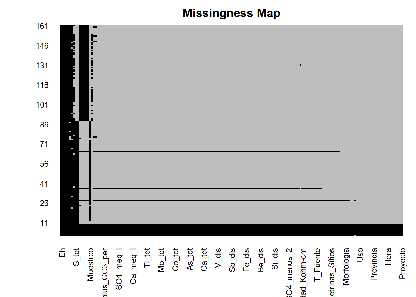
The majority of columns (variables) have 9 rows of null data (we have some variables below and above but we are not going to analyzed that data) so we are going to delete information that not have this data or is empty.
- Delete information that do not have the variable Temporada
Verify the null per Temporada with the function which() and is.na(), then delete this null values from the data frame.
id <- which(is.na(AC$Temporada))
AC <- AC[-id, ]
# check
is.na(AC$Temporada)
## [1] FALSE FALSE FALSE FALSE FALSE FALSE FALSE FALSE FALSE FALSE FALSE FALSE
## [13] FALSE FALSE FALSE FALSE FALSE FALSE FALSE FALSE FALSE FALSE FALSE FALSE
## [25] FALSE FALSE FALSE FALSE FALSE FALSE FALSE FALSE FALSE FALSE FALSE FALSE
## [37] FALSE FALSE FALSE FALSE FALSE FALSE FALSE FALSE FALSE FALSE FALSE FALSE
## [49] FALSE FALSE FALSE FALSE FALSE FALSE FALSE FALSE FALSE FALSE FALSE FALSE
## [61] FALSE FALSE FALSE FALSE FALSE FALSE FALSE FALSE FALSE FALSE FALSE FALSE
## [73] FALSE FALSE FALSE FALSE FALSE FALSE FALSE FALSE FALSE FALSE FALSE FALSE
## [85] FALSE FALSE FALSE FALSE FALSE FALSE FALSE FALSE FALSE FALSE FALSE FALSE
## [97] FALSE FALSE FALSE FALSE FALSE FALSE FALSE FALSE FALSE FALSE FALSE FALSE
## [109] FALSE FALSE FALSE FALSE FALSE FALSE FALSE FALSE FALSE FALSE FALSE FALSE
## [121] FALSE FALSE FALSE FALSE FALSE FALSE FALSE FALSE FALSE FALSE FALSE FALSE
## [133] FALSE FALSE FALSE FALSE FALSE FALSE FALSE FALSE FALSE FALSE FALSE FALSE
## [145] FALSE FALSE FALSE FALSE FALSE FALSE FALSE FALSEError - Ionic Balance
The revision of majoritary analytes (taking to ionic balance) is done in dissolve elements, because is necessary a almost coloidal state, if the filters of sample are small is better.
The equation of Ionic Balance Error is take from Zekâi Şen:
\[Error = \frac{Total Cations - Total Anions}{Total Cations + Total Anions}\]
First we have to convert to meq/l:
# Code to generate equivalents (will not be used, only is mentioned):
# because we have to do data cleansing.
AC$Ca_meq.l <- (AC$Ca_tot*2)/40.08
AC$Mg_meq.l <- (AC$Mg_tot*2)/24.32
AC$Na_meq.l <- (AC$Na_tot*1)/23.00
AC$K_meq.l <-(AC$K_tot*1)/39.10
AC$Cl_meq.l <-(AC$Cl*1)/35.56
AC$SO4_meq.l <-(AC$SO4_menos_2*2)/96.06
AC$HCO3_meq.l <- (AC$HCO3_menos*1)/61.01
AC$CO3_meq.l <- (AC$CO3_menos_2_mg_L*2)/60

AC$Tot_Cat <- rowSums(AC[ ,c("Ca_meq.l","Mg_meq.l","Na_meq.l","K_meq.l")])
AC$Tot_Ani <- rowSums(AC[ ,c("Cl_meq.l","SO4_meq.l","HCO3_meq.l", "CO3_meq.l")])
AC$Err_Rel <- 100*((AC$Tot_Cat-AC$Tot_Ani)/(AC$Tot_Cat+AC$Tot_Ani))
Rename some variables from the data frame and calculate the porcenptual error following the equation mentioned above.
AC <- AC %>% rename(Tot_Cat="Total_meq_l.1", Tot_Ani="Total_meq_l.2")
AC$Error <- 100*((AC$Tot_Cat-AC$Tot_Ani)/(AC$Tot_Cat+AC$Tot_Ani))
Error Analysis with Normality and QQ-Plot:
For the normality test associate with QQ-Plot we are going to use the library ggpubr and ggplot2.
library(ggpubr)
par(mfrow=c(1,2))
qq<-ggplot(AC, aes(sample=Error))+
  geom_qq_line(line.p = c(0.25, 0.75), col = "steelblue")+
  stat_qq()+
  xlab("Cuantiles Teoricos Normales") + ylab("Valores de Error Reales")+
  labs(caption = "Basado en Data del Laboratorio de INGEMMET")+
  scale_colour_manual()

dh <- ggplot(AC, aes(x=Error)) +
  geom_histogram(aes(y = stat(density)), color="black",fill="steelblue") +
  stat_function(
    fun = dnorm,
    args = list(mean = mean(0), sd = sd(AC$Error)),
    lwd = 2,
    col = 'red')+
  geom_vline(xintercept = c(-10,10), linetype="longdash",color="blue",size=1.5)+
  annotate("text", x=2, y=0.12, label="Normal Distribution", color="red", fontface=2,
           size=4)+
  geom_segment(x = 6.4, y = 0.115, xend = 2.2, yend = 0.09,
               arrow = arrow(length = unit(0.5, "cm")))+
  annotate("text",x=-7.5,y=0.13,label="Limite Inferior",color="black", fontface=2,
           size=4)+
  annotate("text",x=+6.0,y=0.13,label="Limite Superior",color="black", fontface=2,
           size=4)

figure <- ggarrange(dh, qq,
                    labels = c("Distribucion de Errores", "QQplot-Errores"),
                    ncol = 2, nrow = 1)
figure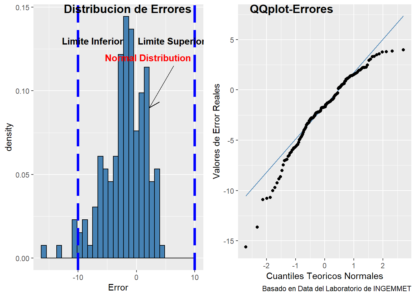
From the picture above we can see the distribution of errors follow pseudo normal distribution, moreover the values of histogram are inside the absolute value of +/-10%. The QQplot-Errores present some tails that not follow a normal distribution. To check that values outside the range we continue with the following code.
Identifying Values outsite of limit
Check the values that are major to 10 % of absolute value. See the code below.
library(DT)
id <- which(AC$Error>=10 | AC$Error<=-10)
datatable(AC[id, ] %>% select(Codigo))
Let´s go to complete values below detection limit 😄
Below Detection Limit Values (<L.D.).
To input values below the detection limit we are going to use the semiparametric method ROS(Robust Regression Orden in Statistics) created by D.R. Helsel and R.M. Hirsch using the NADA (Not Available Data Analysis) (https://cran.r-project.org/web/packages/NADA/index.html) to complete data below detection limit with only one value below the limit, in this case we are going to focus by “temporada” in the sub basin Alto Camaná. We will use the variable Arsenic (As) like example to complete data. The library DT help us to visualization of interactive html table, with tons of options for customization like excel program.
library(DT)
# Will filter Temporada equal to Avenida
datatable(AC[ ,c("As_dis", "Cu_dis")], filter = "top")
As you can see the table above have on the left the dissolved Arsenic value below the detecction limit <0.001 and on the right the dissolved Copper value below the detection limit <0.0005. So we are goint to complet this data in order to use this variable values and not loose the information of the rows for make multivariable analysis. Adittionally, we have to use criteria tu complete the data following two principals things :
Spatial Distribution of the Sample.
Temporal Distribution of the Sample.
Geological Domain of the Sample.
That 3 factors mentioned above can change drastically the way to input values, so we have to take in consideration.
library(DT)
z <- AC[AC$Temporada=="Avenida", ] #Do it the same for Estiaje
#Preparing Data for Analysis:
val0 <- unique(grep("<", z$As_dis, value = TRUE))
z$var0 <- z$As_dis
z$ND_var0 <- rep(0, length(z$var0))
indcero0 <- which(z$var0==val0)
z$var0[indcero0] <- substr(val0,2,nchar(val0))
z$var0 <- as.numeric(z$var0)
z$ND_var0[indcero0] <- 1
z$ND_var0 <- as.logical(z$ND_var0)
#Sort the Data Acorder to Study:
indna0 <- is.na(z$var0)
yn0 <- z$var0[which(indna0==FALSE)]
cyn0 <- z$ND_var0[which(indna0==FALSE)]
yn0 <- sort(yn0,index.return=TRUE)
cyn0 <- cyn0[yn0$ix]
#Apply the ROS (REGRESSION IN ORDER STATISTICS)
elemento <- ros(yn0$x,cyn0,forwardT = "log", reverseT = "exp")
elemento <- as.data.frame(elemento)
id <- which(elemento$censored==TRUE)
elemento <-  elemento[id, ]

#Do it carefully!!!!
AC$As_com <- AC$As_dis #omit this step in estiaje

#Loop to Imput Values:
id <- which(AC$As_com==val0)

for(i in 1:length(id)){
      replace <- elemento$modeled[i]
      AC[id, ]$As_com[i] <-  replace
}

#Do it the same for Estiaje:
z <- AC[AC$Temporada=="Estiaje", ] #
#Preparing Data for Analysis:
val0 <- unique(grep("<", z$As_dis, value = TRUE))
z$var0 <- z$As_dis
z$ND_var0 <- rep(0, length(z$var0))
indcero0 <- which(z$var0==val0)
z$var0[indcero0] <- substr(val0,2,nchar(val0))
z$var0 <- as.numeric(z$var0)
z$ND_var0[indcero0] <- 1
z$ND_var0 <- as.logical(z$ND_var0)
#Sort the Data Acorder to Study:
indna0 <- is.na(z$var0)
yn0 <- z$var0[which(indna0==FALSE)]
cyn0 <- z$ND_var0[which(indna0==FALSE)]
yn0 <- sort(yn0,index.return=TRUE)
cyn0 <- cyn0[yn0$ix]
#Apply the ROS (REGRESSION IN ORDER STATISTICS)
elemento <- ros(yn0$x,cyn0,forwardT = "log", reverseT = "exp")
elemento <- as.data.frame(elemento)
id <- which(elemento$censored==TRUE)
elemento <-  elemento[id, ]

#Loop to Input Values:
id <- which(AC$As_com==val0)

for(i in 1:length(id)){
      replace <- elemento$modeled[i]
      AC[id, ]$As_com[i] <-  replace
}

#Finally run this:
AC$As_com <- as.numeric(AC$As_com)
datatable(AC[ ,c("As_dis","As_com")])  #Test if works
Well, is done! 😀
Exploratory Data Analysis usign statistics
First we need the caracters convert into factors, moreover select the most important columns to develop the analysis (this last depend a lot of geological criteria and the object that you wish), although is an exploratory data analysis, so let´s go all in!! 😄
- Loading data with complet elements values (after ROS)
AC_final <- read.csv(file = "BD_AC_final.csv", header = TRUE)
# sapply(AC , class) see variables class
Convert characters to factors:
Select variable to convert into factors:
cols <- c("Proyecto","Temporada","Codigo","Codigo_Corto","Nombre",
          "Nombre_Completo","Zona","Lugar","Distrito","Provincia",
          "Vertiente","Cuenca","Subcuenca","Microcuenca",
          "Tipo_Fuente","Clase_Fuente","Uso","Asp_Geologico","Desc_Litologica",
          "Morfologia","Color","Olor","Precipitados","Algas_plantas","Basurales",
          "Animales","Letrinas_Sítios","Poblacion","Pasivos_Ambientales","Act_Antropica",
          "Alt.Geo.Nat","Ev.Meteo","Viento","Foto","Observaciones","Realizado_por")
AC_final[cols] <- lapply(AC_final[cols], factor)
Summary Information:
summary(AC_final[ ,-1]) # The first column was create automatically (omit)## Proyecto Temporada Codigo Codigo_Corto Nombre
## GA47C:152 Avenida:73 13491-19-GW-121: 2 GW-121 : 2 Colca :42
## Estiaje:79 13491-19-GW-134: 2 GW-134 : 2 Parhuayune: 8
## 13491-19-GW-138: 2 GW-138 : 2 Challecone: 6
## 13491-19-GW-141: 2 GW-141 : 2 Japo : 5
## 13491-19-GW-146: 2 GW-146 : 2 Challacone: 4
## 13491-19-GW-149: 2 GW-149 : 2 Chila : 4
## (Other) :140 (Other):140 (Other) :83
## Nombre_Completo Fecha Hora
## Río Colca :42 Length:152 Length:152
## Quebrada Parhuayune: 6 Class :character Class :character
## Quebrada Chimpa : 4 Mode :character Mode :character
## Quebrada Escalera : 4
## Quebrada Llaquipaya: 4
## Río Challecone : 4
## (Other) :88
## Norte Este Cota Zona
## Min. :8262499 Min. :178150 Min. :2103 18 S: 1
## 1st Qu.:8268781 1st Qu.:200592 1st Qu.:3328 19 S:151
## Median :8273388 Median :214990 Median :3563
## Mean :8274788 Mean :211382 Mean :3566
## 3rd Qu.:8280416 3rd Qu.:222612 3rd Qu.:3849
## Max. :8291173 Max. :235437 Max. :4565
##
## Lugar Distrito Provincia Vertiente
## Belén : 6 Chivay :29 Caylloma:152 Pacífico:152
## Florida : 6 Tuti :27
## La Calera : 5 Madrigal :23
## Tuti : 5 Achoma :14
## Ancoccollo : 4 Coporaque:14
## Campamento Minero: 4 Maca :10
## (Other) :122 (Other) :35
## Cuenca Subcuenca Microcuenca Tipo_Fuente
## Camaná:152 Alto Camaná:152 Cabanaconde:35 Subterránea: 28
## Maca :53 Superficial:124
## Tuti :64
##
##
##
##
## Clase_Fuente Uso PFQ
## Galería : 5 Ninguno :62 Length:152
## Galería Filtrante: 1 Agropecuario :33 Class :character
## Geiser : 2 Ganadería :16 Mode :character
## Manantial :10 Agropecuario, Consumo humano:10
## Quebrada :61 Balneológico : 9
## Río :63 Agrícola : 8
## Termal :10 (Other) :14
## T.Analisis Muestreo Monitoreo Blanco
## Length:152 Length:152 Length:152 Mode:logical
## Class :character Class :character Class :character NA's:152
## Mode :character Mode :character Mode :character
##
##
##
##
## Estandar Duplicado
## Mode:logical Length:152
## NA's:152 Class :character
## Mode :character
##
##
##
##
## Asp_Geologico
## Volcánico/Depósito superficial :72
## Depósito superficial :32
## Volcánico/Sedimentario/Depósito superficial:19
## Sedimentario/Depósito superficial :14
## Volcánico :10
## (Other) : 4
## NA's : 1
## Desc_Litologica
## Ambos márgenes lavas volcánicas, en el lecho del río depósitos de cantos de bloque de 10 cm hasta 3 m de diámetro. En el lecho del río los bloques están cubiertos de arenas finas, medias y gruesas. : 2
## Básicamente el entorno geológico de este punto de muestreo está constituido por un depósito cuaternario (cantos y bloques polimícticos de hasta 1 m de diámetro ) y suelo orgánico en la superficie de las márgenes de la quebrada: 2
## El entorno geológico de este manantial, son depósitos cuaternarios de la Fm. Colca dispuestos en un sistema de andenería. Al sur del punto de muestras tenemos depósitos de conglomerados que corresponden a la Fm. Colca. : 2
## El entorno geológico de este punto se limita a depósitos cuaternarios (dispuestos en terrazas o sistemas de andenes). Al suroeste del punto (a más de 50 metros aproximadamente) tenemos conglomerados de la Fm. Colca. : 2
## El entorno geológico en el punto de muestreo, son depósitos cuaternarios. En la parte superior (al sureste) se observa tobas andesíticas piroclásticas que corresponden al Complejo Volcánico del Mismi. : 2
## (Other) :141
## NA's : 1
## Morfologia Pendiente Caudal
## Valle :30 Length:152 Min. : 2.50
## Valle Fluvial :28 Class :character 1st Qu.: 26.25
## Quebrada :22 Mode :character Median : 100.00
## Valle encañonado:17 Mean : 979.65
## Cañón :15 3rd Qu.:1150.00
## (Other) :39 Max. :5000.00
## NA's : 1 NA's :116
## Color Olor T_Fuente
## Incoloro :123 Fétido : 2 Min. : 6.00
## Verdoso : 8 Inodoro :141 1st Qu.:12.50
## ligeramente amarillento: 5 Ligeramente\nsulfuroso: 1 Median :15.60
## Amarillento : 3 sulfuroso : 2 Mean :18.21
## Beige : 2 Sulfuroso : 3 3rd Qu.:18.90
## (Other) : 8 NA's : 3 Max. :85.50
## NA's : 3 NA's :3
## T_Ambiente pH pH_mV Eh ORP_mv
## Mode:logical Min. :4.300 Min. : 0.10 Mode:logical Min. : 23.3
## NA's:152 1st Qu.:7.390 1st Qu.: 33.60 NA's:152 1st Qu.:160.7
## Median :8.030 Median : 60.90 Median :222.6
## Mean :7.834 Mean : 60.02 Mean :229.7
## 3rd Qu.:8.490 3rd Qu.: 79.80 3rd Qu.:285.3
## Max. :9.370 Max. :173.00 Max. :523.7
## NA's :3 NA's :3 NA's :3
## CE_uS_cm TDS_mg_L TDS_ppt Salinidad_PSU
## Min. : 55.92 Min. : 27.94 Min. :1.898 Min. :0.0750
## 1st Qu.: 196.20 1st Qu.: 96.78 1st Qu.:2.018 1st Qu.:0.1440
## Median : 438.60 Median : 215.40 Median :2.566 Median :0.2590
## Mean : 730.81 Mean : 358.56 Mean :2.678 Mean :0.4177
## 3rd Qu.: 672.20 3rd Qu.: 326.30 3rd Qu.:3.383 3rd Qu.:0.3690
## Max. :7188.00 Max. :3523.00 Max. :3.523 Max. :3.9840
## NA's :3 NA's :3 NA's :147 NA's :3
## Resistividad_Kohm.cm OD_mgL OD_Sat. Precipitados
## Min. : 0.1391 Min. :1.140 Min. : 12.6 No :134
## 1st Qu.: 1.5050 1st Qu.:6.410 1st Qu.:101.5 Si : 7
## Median : 2.2730 Median :7.030 Median :106.4 Si (óxidos de Fe) : 3
## Mean : 3.8713 Mean :6.814 Mean :105.9 Si (sulfatos) : 1
## 3rd Qu.: 5.0840 3rd Qu.:7.680 3rd Qu.:112.9 Si (sulfuros) : 1
## Max. :17.8400 Max. :9.090 Max. :161.8 Si, Óxidos de \nFe: 4
## NA's :3 NA's :7 NA's :7 NA's : 2
## Algas_plantas Basurales Animales Letrinas_Sítios
## No :108 No :137 no : 1 no : 40
## Sí : 24 NO : 1 nO : 1 No :106
## Sí (abundante) : 6 Sí : 11 No :104 Sí : 4
## Si (algas verdes): 3 Sí (poco): 1 Sí : 44 NA's: 2
## Sí (algas verdes): 3 NA's : 2 NA's: 2
## (Other) : 6
## NA's : 2
## Poblacion Pasivos_Ambientales Act_Antropica
## Rural :146 no :52 Ninguno :76
## Urbana: 3 No :96 Agropecuario :32
## NA's : 3 NO : 1 Ganadería :23
## Sí : 1 Mina abandonada:12
## NA's: 2 Mina Paralizada: 2
## (Other) : 5
## NA's : 2
## Alt.Geo.Nat
## No :120
## Sí : 11
## Sí (presencia de óxidos) : 5
## Sí (aguas arriba) : 3
## Sí (coloración rojizo de lavas volcánicas): 2
## (Other) : 10
## NA's : 1
## Ev.Meteo Viento
## Llovió y granizó \ndias antes (en nacientes): 1 No :101
## Llovió y granizo en \npartes altas : 1 Sí, leve : 16
## Lluvia ligera : 1 Sí, moderado : 15
## Lluvia un dia antes cabecera : 5 Si (Leve a Moderado): 9
## Ninguno :138 Sí : 4
## Poblador indicó que \nllovio dias antes. : 4 (Other) : 5
## NA's : 2 NA's : 2
## Foto
## 669677 : 2
## 10331043: 1
## 10441055: 1
## 10561070: 1
## 10861098: 1
## (Other) :108
## NA's : 38
## Observaciones
## Ninguna :61
## Es captado con canal para el regadío de plantaciones : 2
## La quebrada en esta época del año (temporada de estiaje) se encontró seca. : 2
## Tenemos presencia antrópica y evidencia de basurales a los alrededores del punto de muestreo. : 2
## 3 tuberías de 6 pulgadas cada una que nos da un caudal aproximado de 50 l/s. Se captan varias tuberías desde la boca de la galería (captación para Cabanaconde), aguas abajo tenemos una represa de regadío de 100 metros aproximadamente. : 1
## 3 tuberías de 6 pulgadas cada una que nos da un caudal aproximado de 50 l/s. Se captan varias tuberías desde la boca de la galería (captación para\n Cabanaconde), aguas abajo tenemos una represa de regadío de 100 metros aproximadamente.: 1
## (Other) :83
## Realizado_por Alcalinidad_mgCaCO3_L
## J. Moreno y M. Huaripata :37 Length:152
## I. Becerra y J. Ortiz :36 Class :character
## J.Ortiz & A.Otiniano :26 Mode :character
## M.Carrasco & I. Becerra :26
## M. Huaripata & J. Andrade :24
## J. Ortiz, M. Huaripata & A. Otiniano: 1
## (Other) : 2
## CO3_menos_2_mg_L HCO3_menos F Cl
## Length:152 Length:152 Length:152 Length:152
## Class :character Class :character Class :character Class :character
## Mode :character Mode :character Mode :character Mode :character
##
##
##
##
## NO3_menos_1 NO3_menos_1_como_N SO4_menos_2 NO2_menos_1
## Length:152 Length:152 Min. : 2.854 Length:152
## Class :character Class :character 1st Qu.: 21.200 Class :character
## Mode :character Mode :character Median : 40.200 Mode :character
## Mean : 94.927
## 3rd Qu.:131.700
## Max. :731.700
## NA's :3
## NO2_menos_1_como_N Na_dis Mg_dis K_dis
## Length:152 Min. : 1.96 Min. : 0.600 Min. : 0.700
## Class :character 1st Qu.: 6.30 1st Qu.: 3.977 1st Qu.: 2.400
## Mode :character Median : 16.10 Median : 5.527 Median : 4.100
## Mean : 85.22 Mean : 7.611 Mean : 8.436
## 3rd Qu.: 59.05 3rd Qu.: 9.300 3rd Qu.: 6.300
## Max. :1414.00 Max. :47.490 Max. :89.600
## NA's :3 NA's :3 NA's :3
## Ca_dis Sr_dis Li_dis Si_dis
## Min. : 2.60 Min. :0.0250 Length:152 Min. : 6.10
## 1st Qu.: 15.09 1st Qu.:0.1274 Class :character 1st Qu.:10.30
## Median : 21.70 Median :0.3582 Mode :character Median :13.97
## Mean : 34.08 Mean :0.4566 Mean :18.10
## 3rd Qu.: 41.70 3rd Qu.:0.5412 3rd Qu.:19.90
## Max. :176.50 Max. :4.4601 Max. :93.50
## NA's :3 NA's :3 NA's :3
## SiO2._dis Ag_dis Al_dis As_dis
## Min. : 13.05 Length:152 Length:152 Length:152
## 1st Qu.: 22.04 Class :character Class :character Class :character
## Median : 29.90 Mode :character Mode :character Mode :character
## Mean : 38.74
## 3rd Qu.: 42.59
## Max. :200.09
## NA's :3
## B_dis Ba_dis Be_dis Bi_dis
## Length:152 Min. :0.00320 Length:152 Length:152
## Class :character 1st Qu.:0.02190 Class :character Class :character
## Mode :character Median :0.03190 Mode :character Mode :character
## Mean :0.03441
## 3rd Qu.:0.04060
## Max. :0.13550
## NA's :3
## Cd_dis Ce_dis Co_dis Cr_dis
## Length:152 Length:152 Length:152 Length:152
## Class :character Class :character Class :character Class :character
## Mode :character Mode :character Mode :character Mode :character
##
##
##
##
## Cu_dis Fe_dis Hg_dis La_dis
## Length:152 Length:152 Length:152 Length:152
## Class :character Class :character Class :character Class :character
## Mode :character Mode :character Mode :character Mode :character
##
##
##
##
## Mn_dis Mo_dis Ni_dis Pb_dis
## Length:152 Length:152 Length:152 Length:152
## Class :character Class :character Class :character Class :character
## Mode :character Mode :character Mode :character Mode :character
##
##
##
##
## S_dis Sb_dis Se_dis Sn_dis
## Min. : 1.20 Length:152 Length:152 Length:152
## 1st Qu.: 5.10 Class :character Class :character Class :character
## Median : 11.10 Mode :character Mode :character Mode :character
## Mean : 25.94
## 3rd Qu.: 22.00
## Max. :245.10
## NA's :79
## Th_dis Ti_dis Tl_dis U_dis
## Length:152 Length:152 Length:152 Length:152
## Class :character Class :character Class :character Class :character
## Mode :character Mode :character Mode :character Mode :character
##
##
##
##
## V_dis W_dis Y_dis Zn_dis
## Length:152 Length:152 Length:152 Length:152
## Class :character Class :character Class :character Class :character
## Mode :character Mode :character Mode :character Mode :character
##
##
##
##
## Na_tot Mg_tot K_tot Ca_tot
## Min. : 2.00 Min. : 0.600 Min. : 0.700 Min. : 2.71
## 1st Qu.: 6.60 1st Qu.: 4.185 1st Qu.: 2.600 1st Qu.: 15.40
## Median : 17.60 Median : 6.300 Median : 4.500 Median : 22.60
## Mean : 92.43 Mean : 8.236 Mean : 8.857 Mean : 35.70
## 3rd Qu.: 63.70 3rd Qu.: 9.766 3rd Qu.: 7.000 3rd Qu.: 42.83
## Max. :1436.00 Max. :47.490 Max. :89.600 Max. :182.30
## NA's :3 NA's :3 NA's :3 NA's :3
## Sr_tot Li_tot Si_tot SiO2_tot
## Min. :0.0250 Length:152 Min. : 6.70 Min. : 14.34
## 1st Qu.:0.1318 Class :character 1st Qu.: 12.01 1st Qu.: 25.70
## Median :0.3605 Mode :character Median : 16.31 Median : 34.90
## Mean :0.4799 Mean : 20.01 Mean : 42.82
## 3rd Qu.:0.5447 3rd Qu.: 21.00 3rd Qu.: 44.94
## Max. :5.0821 Max. :101.54 Max. :217.30
## NA's :3 NA's :3 NA's :3
## Ag_tot Al_tot As_tot B_tot
## Length:152 Length:152 Length:152 Length:152
## Class :character Class :character Class :character Class :character
## Mode :character Mode :character Mode :character Mode :character
##
##
##
##
## Ba_tot Be_tot Bi_tot Cd_tot
## Min. :0.00270 Length:152 Length:152 Length:152
## 1st Qu.:0.02120 Class :character Class :character Class :character
## Median :0.03300 Mode :character Mode :character Mode :character
## Mean :0.03629
## 3rd Qu.:0.04450
## Max. :0.14850
## NA's :3
## Ce_tot Co_tot Cr_tot Cu_tot
## Length:152 Length:152 Length:152 Length:152
## Class :character Class :character Class :character Class :character
## Mode :character Mode :character Mode :character Mode :character
##
##
##
##
## Fe_tot Hg_tot La_tot Mn_tot
## Length:152 Length:152 Length:152 Length:152
## Class :character Class :character Class :character Class :character
## Mode :character Mode :character Mode :character Mode :character
##
##
##
##
## Mo_tot Ni_tot Pb_tot S_tot
## Length:152 Length:152 Length:152 Min. : 1.40
## Class :character Class :character Class :character 1st Qu.: 6.10
## Mode :character Mode :character Mode :character Median : 13.10
## Mean : 29.94
## 3rd Qu.: 24.40
## Max. :286.00
## NA's :79
## Sb_tot Se_tot Sn_tot Th_tot
## Length:152 Length:152 Length:152 Length:152
## Class :character Class :character Class :character Class :character
## Mode :character Mode :character Mode :character Mode :character
##
##
##
##
## Ti_tot Tl_tot U_tot V_tot
## Length:152 Length:152 Length:152 Length:152
## Class :character Class :character Class :character Class :character
## Mode :character Mode :character Mode :character Mode :character
##
##
##
##
## W_tot Y_tot Zn_tot Ca_meq_l
## Length:152 Length:152 Length:152 Min. :0.1300
## Class :character Class :character Class :character 1st Qu.:0.7545
## Mode :character Mode :character Mode :character Median :1.0850
## Mean :1.7039
## 3rd Qu.:2.0850
## Max. :8.8250
## NA's :3
## Mg_meq_l Na_meq_l K_meq_l Total_meq_l...156
## Min. :0.04938 Min. : 0.08522 Min. :0.01790 Min. : 0.3806
## 1st Qu.:0.32732 1st Qu.: 0.27391 1st Qu.:0.06138 1st Qu.: 1.5755
## Median :0.45490 Median : 0.70000 Median :0.10486 Median : 3.6996
## Mean :0.62646 Mean : 3.70521 Mean :0.21576 Mean : 6.2513
## 3rd Qu.:0.76543 3rd Qu.: 2.56739 3rd Qu.:0.16113 3rd Qu.: 5.9735
## Max. :3.90864 Max. :61.47826 Max. :2.29156 Max. :66.2801
## NA's :3 NA's :3 NA's :3 NA's :3
## HCO3_meq_l CO3_meq_l SO4_meq_l Cl_meq_l
## Min. : 0.0000 Min. :0.00000 Min. : 0.05946 Min. : 0.0000
## 1st Qu.: 0.6672 1st Qu.:0.00000 1st Qu.: 0.44167 1st Qu.: 0.0141
## Median : 1.2033 Median :0.00000 Median : 0.83750 Median : 0.1044
## Mean : 1.8472 Mean :0.08723 Mean : 1.97765 Mean : 2.7409
## 3rd Qu.: 1.6557 3rd Qu.:0.03333 3rd Qu.: 2.74375 3rd Qu.: 2.2087
## Max. :23.3443 Max. :1.56000 Max. :15.24375 Max. :45.8110
## NA's :3 NA's :3 NA's :3 NA's :3
## Total_meq_l...161 BI_per Ca_per Mg_per
## Min. : 0.4094 Min. :-15.5923 Min. : 4.602 Min. : 0.4133
## 1st Qu.: 1.7281 1st Qu.: -3.8192 1st Qu.:26.086 1st Qu.: 9.9555
## Median : 3.8016 Median : -1.6729 Median :35.069 Median :16.7539
## Mean : 6.6530 Mean : -2.0072 Mean :39.596 Mean :17.1872
## 3rd Qu.: 6.2555 3rd Qu.: 0.6315 3rd Qu.:49.767 3rd Qu.:24.4770
## Max. :73.0932 Max. : 3.9943 Max. :82.072 Max. :39.8120
## NA's :3 NA's :3 NA's :3 NA's :3
## Na_plus_K_per HCO3_plus_CO3_per SO4_per Cl_per
## Min. : 4.878 Min. : 0.00 Min. : 7.714 Min. : 0.000
## 1st Qu.:22.967 1st Qu.:29.40 1st Qu.: 14.146 1st Qu.: 1.049
## Median :40.442 Median :36.98 Median : 24.660 Median : 4.142
## Mean :43.217 Mean :43.00 Mean : 35.155 Mean :21.841
## 3rd Qu.:62.009 3rd Qu.:65.05 3rd Qu.: 45.032 3rd Qu.:46.516
## Max. :94.176 Max. :90.59 Max. :100.000 Max. :76.526
## NA's :3 NA's :3 NA's :3 NA's :3
## HIDROTIPO As_com As_ran B_com
## Length:152 Min. :0.0000405 Length:152 Min. : 0.000383
## Class :character 1st Qu.:0.0013000 Class :character 1st Qu.: 0.022420
## Mode :character Median :0.0058000 Mode :character Median : 0.080000
## Mean :0.0530550 Mean : 1.213220
## 3rd Qu.:0.0266000 3rd Qu.: 0.520000
## Max. :1.7420000 Max. :24.330000
## NA's :3 NA's :3
## B_ran Cu_com Cu_ran Fe_com
## Length:152 Min. :0.000122 Length:152 Min. :0.00122
## Class :character 1st Qu.:0.001200 Class :character 1st Qu.:0.02000
## Mode :character Median :0.001800 Mode :character Median :0.03500
## Mean :0.038542 Mean :0.08423
## 3rd Qu.:0.002800 3rd Qu.:0.09000
## Max. :4.597300 Max. :0.79100
## NA's :3 NA's :3
## Fe_ran Mn_com Mn_ran pH_ran
## Length:152 Min. :0.000043 Length:152 Length:152
## Class :character 1st Qu.:0.003100 Class :character Class :character
## Mode :character Median :0.010400 Mode :character Mode :character
## Mean :0.192173
## 3rd Qu.:0.032600
## Max. :6.787600
## NA's :3
## CE_ran Ti_com Ti_ran Zn_com
## Length:152 Min. :0.00022 Length:152 Min. : 0.0002
## Class :character 1st Qu.:0.00130 Class :character 1st Qu.: 0.0050
## Mode :character Median :0.00190 Mode :character Median : 0.0080
## Mean :0.00341 Mean : 2.4203
## 3rd Qu.:0.00360 3rd Qu.: 0.0320
## Max. :0.04630 Max. :95.4800
## NA's :75 NA's :64
## Zn_ran Ni_com Ni_ran
## Length:152 Min. :0.00000 Length:152
## Class :character 1st Qu.:0.00010 Class :character
## Mode :character Median :0.00060 Mode :character
## Mean :0.00278
## 3rd Qu.:0.00135
## Max. :0.04550
## NA's :58You can check carefully the summary, in my case I spend some time understanding the summary variable by variable to try to understand the whole data.
To make the preliminary analysis we are going to use 4 principal factors:
- Temporada.
- Microcuenca.
- Tipo Fuente.
- Clase Fuente.
And inside the qualitative variables:
- The complete elements of As_com, B_com, Cu_com, Fe_com, Mn_com, Ti_com, Ni_com with T_Fuente, pH, ORP_mv, CE_uS_cm, TDS_mg_L, Salinidad_PSU.
We can considerate more variables, more sections, but in this case only will use only the mentions above. Will use a powerful package tidyverse().
GGPLOT
The ggplot package have fully functionality of grammar graphics for data science, so the principal thing that you have to know is the general structure to start using this awesome creation, thanks to Hadley Wickhman & Garrett Grolemund
— A.Otiniano
Structure ggplot
General Structure
This the general structure of ggplot2:
ggplot(data=<DATA>)+
  <GEOM_FUNCTION>(
    mapping=aes(<MAPPINGS>),
    stat=<STAT>,
    position=<POSITION>
  )+
  <COORDINATE_FUNCTION>+
  <FACET_FUNCTION>
Arguments and Functions
aes()
Aesthetics works with arguments that are: x, y, color, shape, size, alpha, linetype, group, fill and wight. That are design to use many variables as you can!
facet()
This mean faces, divide the graph by variables using: facet_wrap() and facet_grid() functions, the fisrt is 1 variable, the second 2 variables, in general.
geom features
The grammar of graphics use geom_smooth(), geom_bar(), geom_boxplot(), geom_histogram(), geom_vline(), geom_hline() and geom_abline() like principals functions to make and exploratory graph analysis.
coordinates
You can flip coordinates using: coord_flip() function, also yoy can use coor_quickmap() for making maps or coor_polar() for make transformation or coord_fixed() to make scale data.
Filter a variable to analyze (pH o CE):
With this brife introduction we can continue with the data analysis, to see more check R for Data Science R4DS.
library(DT)
id <- which(is.na(AC_final$pH))
AC_final <- AC_final[-id, ]
Graphical Analysis:
First we need some libraries additional to tydiverse package:
library(ggpubr); library(ggrepel)
library(ggExtra); library(plotly)
library(ggridges); library(GGally)
To start with the graphical analysis we have to choose some quantitative and qualitative variables, we will choose only a few to make the analysis easier. The variables are hydrogen potencial (pH), electric conductivity (Ce) like quantitative variables, and Temporada (Avenida and Estiaje), Subbasin, Tipo de Fuente (Surface o Subsurface water) and Clase Fuente (Termal, Stream, River, Geiser, Spring, Gallery and filtering Gallery) like qualitative.
We will use Uni-variant and Bi-variant Analysis with factors.
First we take all the sub-basin together, and we will use panel set view to communicate data in easy way.
Graphical 1st Analysis
pH Vs. Temporada-Tipo_Fuente
qplot(sample=pH, data=AC_final, facets = .~Temporada, color=Tipo_Fuente)+
  labs(title="pH by Temporada and Tipo de Fuente",
       y="pH (non-dimensional)")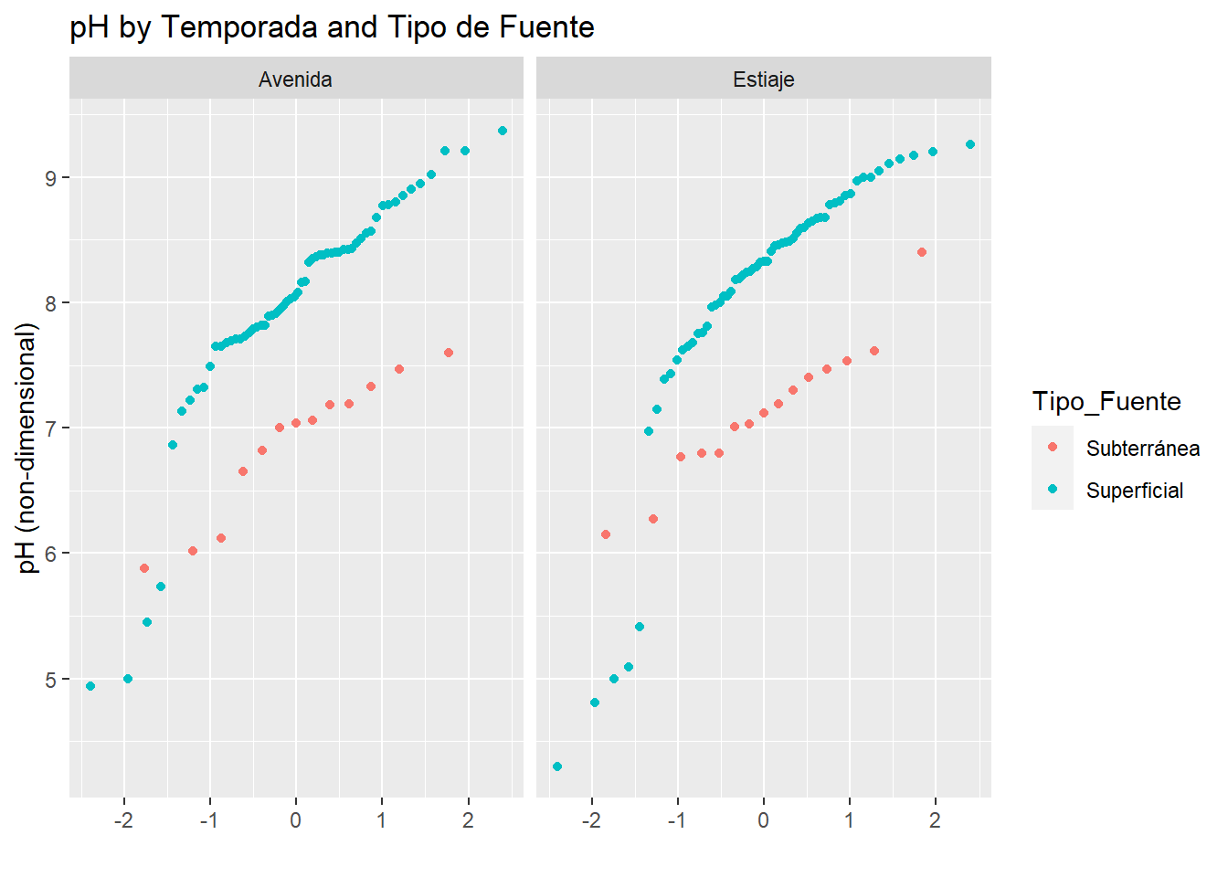
In the picture above we can see that surface (Superficial) water have higher values than subsurface water (Subterránea) in the study area, and slightly tend to grow the values of pH between “Temporada” (higher values in Estiaje).
Ce Vs. Temporada-Tipo_Fuente
qplot(sample=CE_uS_cm, data=AC_final, facets = .~Temporada, color=Tipo_Fuente)+
  labs(title="Ce by Temporada and Tipo de Fuente",
       y="Ce (uS/cm)")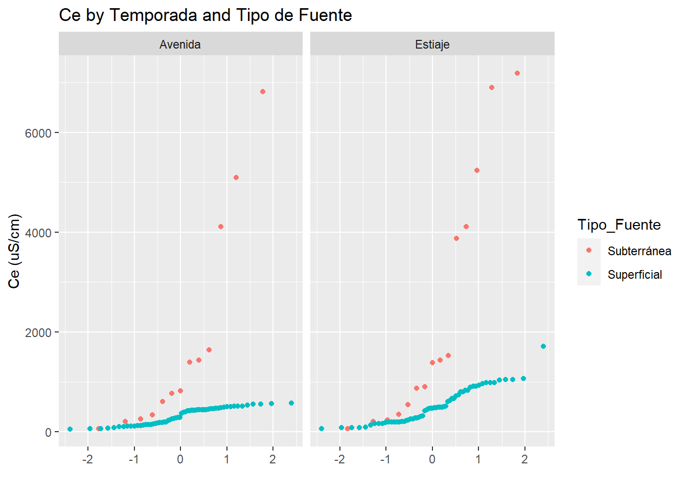
In the uni-variant analysis of electric conductivity we can see a very similar behaivour between surface and subsurface water in both “temporada”
Then we repeat similar code but change qualitative variables, you can analyze that in a similar way (that´s your job 🤠)
pH Vs. Microcuenca-Temporada
qplot(sample=pH, data=AC_final, facets = .~Microcuenca, color=Temporada)+
  labs(title="pH by Temporada and Tipo de Fuente",
       y="pH (non-dimensional)")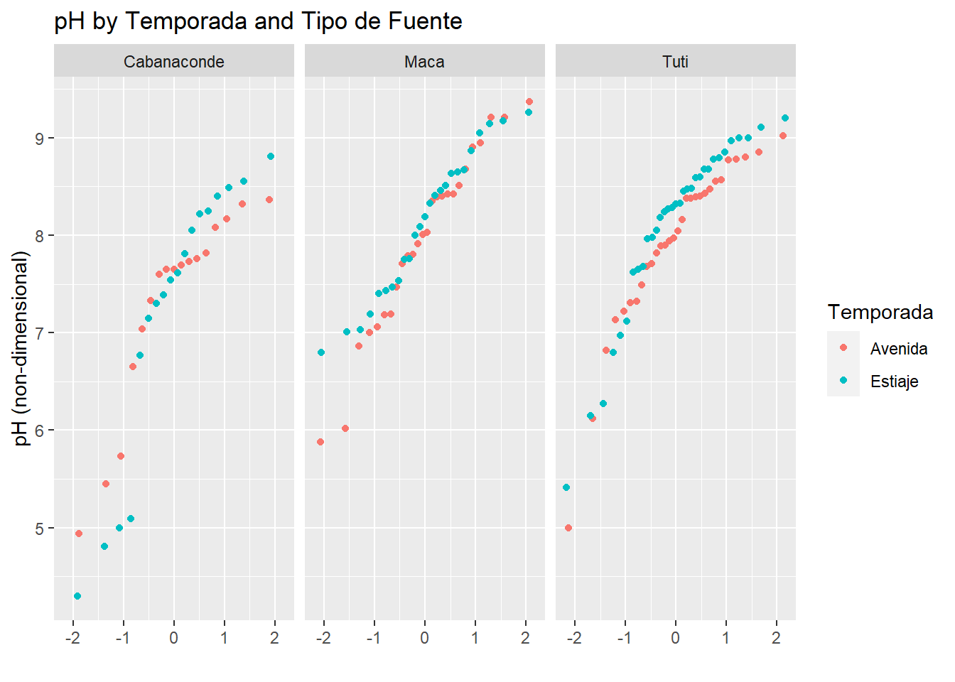
Ce Vs. Microcuenca-Temporada
qplot(sample=CE_uS_cm, data=AC_final, facets = .~Microcuenca, color=Temporada)+
  labs(title="Ce by Temporada and Tipo de Fuente",
       y="Ce (uS/cm)")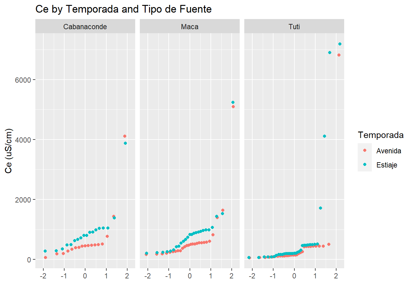
Graphical 2nd Analysis
Then we are going to set the bi-variant analysis:
Univariant pH Distribution
#Library Ridges:
ggplot(AC_final, aes(x=pH, y=Microcuenca))+
  geom_density_ridges(aes(fill=Microcuenca))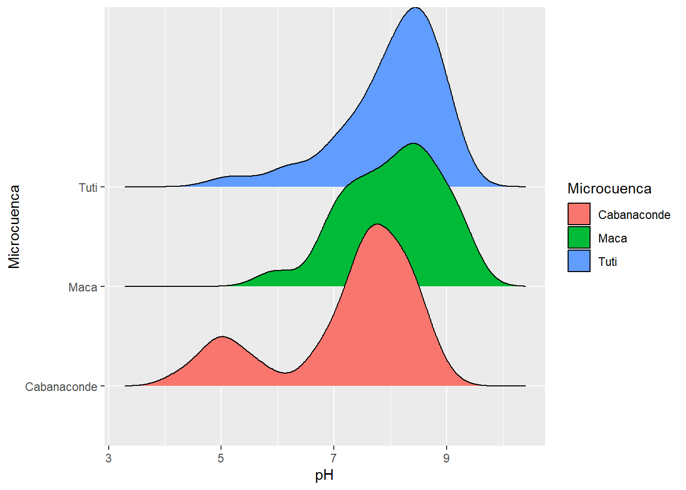
That is not bi-variant, but is important to show you the uni-variant distribution of pH between sub-basins. We can see from the picture that Tuti and Maca have slightly similarities but the Cabanaconde Basin have bi-modal distribution of pH (we can see two peaks in the density distribution for Cabanaconde).
Try to thing what is the reason because Cabanaconde have this behaviour 🤔
Ggplot and Scatterplot
#Scatter e Histograma
ggscatterhist(AC_final, x="pH", y="CE_uS_cm",color="Microcuenca",
              margin.plot = "boxplot",
              ggtheme = theme_bw())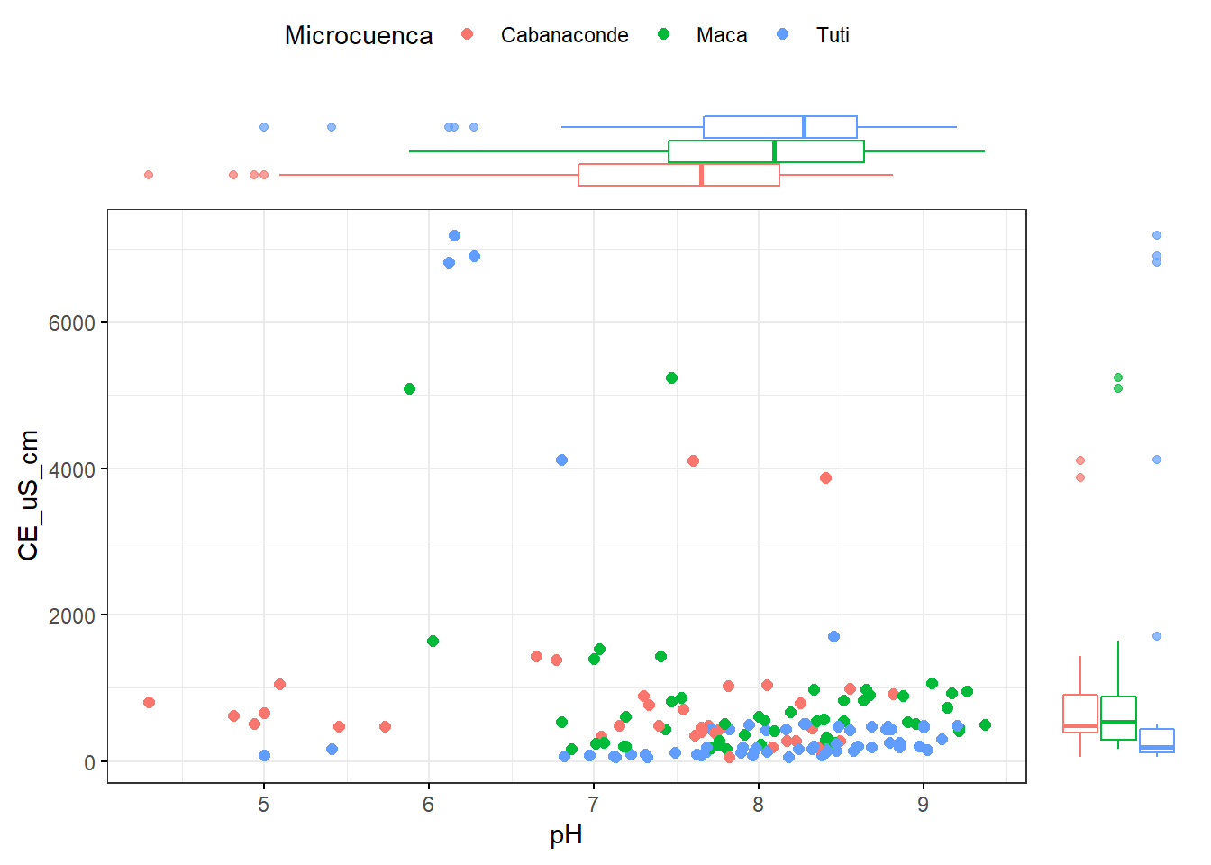
Last but not least, interactive graphs. Well, I am not going to explain the next graphs, but you can interact with these, so I let you try to do it and analyze in your own way, you have the data so do not worry!! 🤓 let´s do it.
Graphical 3erd Analysis
TDS by size
# Graphing TDS according to size:
p <- ggplot(AC_final, aes(x=pH, y=CE_uS_cm, color=Microcuenca))+
  geom_point(aes(size=TDS_mg_L))
ggplotly(p)
Boxplot pH by Temporada
q <- ggplot(AC_final, aes(x=Microcuenca, y=pH, color=Temporada))+
  geom_boxplot(position = position_dodge(0.8))+
  geom_jitter(position = position_dodge(0.8),size=2)+
  scale_color_manual(values = c("steelblue","red"))
ggplotly(q)
Bi-variant analysis pH Vs. Ce with factors Fuente, Temporada and
r <- ggplot(AC_final, aes(x=pH, y=CE_uS_cm, shape = Temporada, color =Microcuenca ))+
  geom_point(size=3.5)+
  facet_grid(.~ Tipo_Fuente)+
  geom_rug()+
  labs(title = "pH Vs. CE (Temporada,Microcuenca,Fuente)")
ggplotly(r)
Boxplot ph by Microcuenca in Alto Camana
p <- ggplot(AC_final, aes(x=Microcuenca, y=pH, fill=Temporada))+
  geom_boxplot()+
  labs(title = "Boxplot de pH por Microcuenca en Alto Camana")+
  facet_grid(.~ Tipo_Fuente )
ggplotly(p)
Point values + statistics
pH_Plot <- ggplot(AC_final, aes(x=Microcuenca, y=pH, color=Temporada))+
  geom_jitter(position=position_jitter(0.2), size=2)+
  facet_grid(.~Temporada)+
labs(title = "Boxplot de pH ")+
  scale_color_manual(values = c("steelblue","red"))+
  theme_minimal()
data_summary<-function(x){
  m <- mean(x)
  ymin <- m-sd(x)
  ymax <- m+sd(x)
  return(c(y=m, ymin=ymin, ymax=ymax))
}
pH_Plot + stat_summary(fun.data = data_summary, color="red")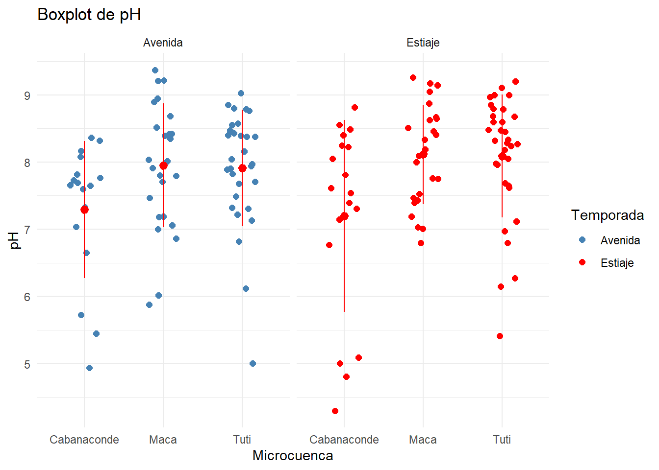
Creating Classification accord to TDS:
Also we can classify the data following some qualitative criteria to change quantitative criteria, we create a TDS_cla variable following the classification of Zekâi Şen.
AC_final$TDS_cla <- with(AC_final,ifelse(TDS_mg_L >= 0 & TDS_mg_L < 200, "Fresh Water",
                           ifelse(TDS_mg_L >= 200 & TDS_mg_L < 500, "Brackish Water"
                                  ,(ifelse(TDS_mg_L>=500 & TDS_mg_L<1500,"Saline Water","Brine Water")))))
AC_final$TDS_cla <- factor(AC_final$TDS_cla, ordered = TRUE)
summary(AC_final$TDS_cla)
## Brackish Water Brine Water Fresh Water Saline Water
## 63 8 67 11We have the new variable classification with the majority between Fresh and Brackish Water, next Saline Water and finally Brine Water.
Multivariable Filters:
We can filter wharever that our mind want to do it, is so is easy with pipelines and tidyverse 😄 so let´s´go to try some filter. You can guess what I want to do.
“Filter 1”
This filtre is preparate to select some variables from the data frame then works like group by Temporada and summarise mean of the selected values.
— A.Otiniano
# Sumario de Media Aritmética de Valores seleccionados por Temporada
Filtro1 <- AC_final %>%
  select(Temporada, As_com, B_com, Cu_com, Fe_com, Mn_com, Ti_com, Ni_com, pH, CE_uS_cm, T_Fuente) %>%
  group_by(Temporada) %>%
  summarise_if(is.numeric, mean, na.rm = TRUE)
Filtro1
## # A tibble: 2 x 11
## Temporada As_com B_com Cu_com Fe_com Mn_com Ti_com Ni_com pH CE_uS_cm
## <fct> <dbl> <dbl> <dbl> <dbl> <dbl> <dbl> <dbl> <dbl> <dbl>
## 1 Avenida 0.0454 0.982 0.0660 0.0639 0.182 0.00345 0.00644 7.78 582.
## 2 Estiaje 0.0604 1.44 0.0122 0.104 0.202 0.00275 0.00191 7.89 874.
## # ... with 1 more variable: T_Fuente <dbl>“Filter 2”
# Sumario de Media Aritmética de Valores seleccionados por Temporada
Filtro2 <- AC_final %>%
  select(Microcuenca, As_com, B_com, Cu_com, Fe_com, Mn_com, Ti_com, Ni_com, pH, CE_uS_cm, T_Fuente) %>%
  group_by(Microcuenca) %>%
  summarise_if(is.numeric, mean, na.rm = TRUE)
Filtro2
## # A tibble: 3 x 11
## Microcuenca As_com B_com Cu_com Fe_com Mn_com Ti_com Ni_com pH CE_uS_cm
## <fct> <dbl> <dbl> <dbl> <dbl> <dbl> <dbl> <dbl> <dbl> <dbl>
## 1 Cabanaconde 0.0937 1.10 0.156 0.129 0.647 0.00231 0.00772 7.24 805.
## 2 Maca 0.0226 1.08 0.00212 0.0538 0.0271 0.00388 0.000335 8.03 786.
## 3 Tuti 0.0551 1.39 0.00263 0.0840 0.0732 0.00364 0.000739 8.00 645.
## # ... with 1 more variable: T_Fuente <dbl>“Filter 3”
# Sumario de Media Aritmética de Valores seleccionados por Temporada
Filtro3 <- AC_final %>%
  select(Tipo_Fuente, As_com, B_com, Cu_com, Fe_com, Mn_com, Ti_com, Ni_com, pH, CE_uS_cm, T_Fuente) %>%
  group_by(Tipo_Fuente) %>%
  summarise_if(is.numeric, mean, na.rm = TRUE)
Filtro3
## # A tibble: 2 x 11
## Tipo_Fuente As_com B_com Cu_com Fe_com Mn_com Ti_com Ni_com pH CE_uS_cm
## <fct> <dbl> <dbl> <dbl> <dbl> <dbl> <dbl> <dbl> <dbl> <dbl>
## 1 Subterránea 0.225 4.97 0.188 0.0606 0.643 0.00918 0.00556 7.01 2086.
## 2 Superficial 0.0133 0.344 0.00401 0.0897 0.0878 0.00224 0.00216 8.03 417.
## # ... with 1 more variable: T_Fuente <dbl>“Filter 4”
# Sumario de Media Aritmética de Valores seleccionados por Temporada
Filtro4 <- AC_final %>%
  select(Clase_Fuente, As_com,Cu_com) %>%
  group_by(Clase_Fuente) %>%
  summarise_if(is.numeric, funs(n(),mean, sd, median))
Filtro4
## # A tibble: 7 x 9
## Clase_Fuente As_com_n Cu_com_n As_com_mean Cu_com_mean As_com_sd Cu_com_sd
## <fct> <int> <int> <dbl> <dbl> <dbl> <dbl>
## 1 Galería 5 5 0.00449 1.04 0.00430 2.00e+0
## 2 Galería Filtra~ 1 1 0.007 0.0006 NA NA
## 3 Geiser 2 2 1.48 0.000172 0.365 3.70e-6
## 4 Manantial 10 10 0.0158 0.00145 0.0252 1.76e-3
## 5 Quebrada 58 58 0.00338 0.00507 0.00431 8.86e-3
## 6 Río 63 63 0.0224 0.00303 0.0203 3.38e-3
## 7 Termal 10 10 0.314 0.00255 0.386 4.69e-3
## # ... with 2 more variables: As_com_median <dbl>, Cu_com_median <dbl>“Filter 5”
Filtro5 <- AC_final %>%
  select(Temporada, As_com, B_com, Cu_com, Fe_com, Mn_com, Ti_com, Ni_com, pH, CE_uS_cm, T_Fuente) %>%
  group_by(Temporada) %>%
summarise_at(.vars = c("pH", "CE_uS_cm"),
               .funs = c(Mean="mean", Median="median", Sd="sd"))
Filtro5
## # A tibble: 2 x 7
## Temporada pH_Mean CE_uS_cm_Mean pH_Median CE_uS_cm_Median pH_Sd CE_uS_cm_Sd
## <fct> <dbl> <dbl> <dbl> <dbl> <dbl> <dbl>
## 1 Avenida 7.78 582. 7.9 402. 0.951 1059.
## 2 Estiaje 7.89 874. 8.20 489. 1.07 1330.“Filter 6”
Filtro6 <- AC_final %>%
  select(Temporada, Microcuenca, Tipo_Fuente,Clase_Fuente, As_com, B_com, Cu_com, Fe_com, Mn_com, Ti_com, Ni_com, pH, CE_uS_cm, T_Fuente) %>%
  filter(pH > 6.5) %>%
  group_by(Temporada, Microcuenca, Tipo_Fuente, Clase_Fuente) %>%
  summarise(
    n = n(),
    mean_As = round(mean(As_com, na.rm = TRUE),4),
    mean_Cu = round(mean(Cu_com, na.rm = TRUE),4)
) %>%
  arrange(desc(n))
datatable(Filtro6, filter = "top")
Like you see you can filter all that you want and in the way that you want, also you can create with datatable() function awesome manilupation of data in html or interactive presentations in web.
Complete Statistic Summary (Quantitative Variables):
Finally, we are going to see a complete statistics summary create by some simple code.
#Appliying to pH and CE mean values.
apply(AC_final[ ,c("pH","CE_uS_cm")],2, mean)
## pH CE_uS_cm
## 7.834027 730.806443estadisticos <- function(x){
Valores <- c(length(x),sum(is.na(x)),min(x, na.rm = TRUE),
quantile(x,probs = 0.25, na.rm = TRUE)-1.5*IQR(x, na.rm = TRUE) ,
quantile(x,probs = 0.25, na.rm = TRUE),
median(x, na.rm = TRUE),mean(x, na.rm = TRUE),mean(x,trim = 0.025, na.rm = TRUE),
quantile(x,probs=0.75, na.rm = TRUE),max(x, na.rm = TRUE),
quantile(x,probs = 0.25, na.rm = TRUE)+1.5*IQR(x, na.rm = TRUE),
IQR(x, na.rm = TRUE), mad(x, na.rm = TRUE),sd(x, na.rm = TRUE),
skew(x, na.rm = TRUE),kurtosi(x, na.rm = TRUE),
CV_CE=(sd(x, na.rm = TRUE)/mean(x, na.rm = TRUE))*100)
}
subset_data <- AC_final %>%
select(Temporada, pH, CE_uS_cm, As_com, B_com, Cu_com, Fe_com, Mn_com, Ni_com) %>%
filter(Temporada=="Estiaje")
colnames(subset_data)## [1] "Temporada" "pH" "CE_uS_cm" "As_com" "B_com" "Cu_com"
## [7] "Fe_com" "Mn_com" "Ni_com"es <- sapply(subset_data[ ,2:9], estadisticos) # 2:9 O -1 funciona igual.
Nombres <- c("n","Vacios","Minimo","LI","Q1","Me:diana","Media","Media Cortada","Q3","Maximo","LS",
"IQR","MAD", "Sd", "As","k", "CV")
rownames(es) <- Nombres
f <- data.frame(es)
#datatable(f) to look fancy.
f## pH CE_uS_cm As_com B_com Cu_com
## n 76.000000 76.000000 76.00000000 76.000000000 7.600000e+01
## Vacios 0.000000 0.000000 0.00000000 0.000000000 0.000000e+00
## Minimo 4.300000 62.800000 0.00004053 0.000494168 1.746962e-04
## LI 5.645000 -806.275000 -0.04393750 -1.538000000 -8.875000e-04
## Q1 7.422500 224.825000 0.00147500 0.025750000 1.400000e-03
## Me:diana 8.205000 489.450000 0.00665000 0.097500000 1.900000e-03
## Media 7.885132 873.680658 0.06041837 1.435727102 1.220451e-02
## Media Cortada 7.915000 799.309865 0.04548318 1.146956292 4.373889e-03
## Q3 8.607500 912.225000 0.03175000 1.068250000 2.925000e-03
## Maximo 9.260000 7188.000000 1.22600000 24.240000000 6.037000e-01
## LS 9.200000 1255.925000 0.04688750 1.589500000 3.687500e-03
## IQR 1.185000 687.400000 0.03027500 1.042500000 1.525000e-03
## MAD 0.859908 446.410860 0.00919212 0.139973142 8.895600e-04
## Sd 1.070086 1330.279177 0.20012579 4.021956197 6.911890e-02
## As -1.369628 3.381815 4.61563768 4.059188641 8.244375e+00
## k 1.751981 11.569382 21.29108387 16.924393255 6.756832e+01
## CV 13.570934 152.261489 331.23334492 280.133751776 5.663392e+02
## Fe_com Mn_com Ni_com
## n 76.000000000 7.600000e+01 7.600000e+01
## Vacios 0.000000000 0.000000e+00 0.000000e+00
## Minimo 0.004063216 5.637423e-05 2.683464e-06
## LI -0.078750000 -4.548750e-02 -1.029105e-03
## Q1 0.027000000 3.075000e-03 6.835799e-05
## Me:diana 0.047500000 1.080000e-02 4.000000e-04
## Media 0.103759667 2.020429e-01 1.906099e-03
## Media Cortada 0.095819885 1.265839e-01 1.438660e-03
## Q3 0.097500000 3.545000e-02 8.000000e-04
## Maximo 0.791000000 5.988000e+00 3.840000e-02
## LS 0.132750000 5.163750e-02 1.165821e-03
## IQR 0.070500000 3.237500e-02 7.316420e-04
## MAD 0.042254100 1.415883e-02 5.165993e-04
## Sd 0.155713383 7.245873e-01 5.594374e-03
## As 2.946222695 6.774496e+00 4.579467e+00
## k 8.539559141 5.058856e+01 2.343642e+01
## CV 150.071205342 3.586304e+02 2.934987e+02write.csv(f, file = "Sumario_Estiaje.csv") #Exportar como .csvConclusions:
The analysis of structure and some exploratory graphs are very useful to start interpretation in water data analysis.
Coding is an efficient way to work with data frame, more with big and complex structures.
We can automatize the analysis through programming language reducing 20 times that we made in a normal way.
Recommendations:
You have considerate the time to learn programming but at the same the huge benefits that you recipe when you know.
Taking step by step learning how to analyze data from water resource.
Explore as much as you can the variables and relation between them.
Bibliography:
The bibliography to go deeper in the evaluation of data is the following:
R for Data Science, ver R4DS, Hands-On Programming with R.
Colección de Paquetes Data Science, ver Tidyverse y listado de paquetes.
Generación de Libros Interactivos, documentos y analisis, ver R Markdown Cookbook, R Markdown: The Definitive Guide, bookdown, Mastering Shiny, Interactive web-based data visualization with R, plotly, and shiny
Rstudio y R, ver Rstudio, Studio Blog, useR.
Journals - Books, ver The R Journal, Chapman & Hall/CRC The R Series, Serie Use R.
Machine Learning, ver Hands-On Machine Learning with R.
Geoquimica, ver Geochemical Modelling of Igneous Processes – Principles And Recipes in R Language, paquetes importantes Geological Survey of Canada - rgr:Applied Geochemestry Data EDA y USGS - GcClust: Clustering regional geochemical data
Hidroquimica, ver CRAN Task View: Hydrological Data and Modeling.